p. 74 · PDF 78

3 - 4 QC (Quality Control) Techniques

QC (Quality Control) techniques are all activities which are carried out to draft and achieve plans for the most economical production of products that sufficiently satisfy customers (or consumers). They are performed according to the PDCA cycle. The key points of quality control are the setting and assuring of specified values (e.g., mean values) for product length, weight, or other characteristics, and the controlling of unevenness in products. These mean values are set in the ISO 9000 series for quality control systems. A variety of mathematical techniques are used to control unevenness in products. Quality control using mathematical techniques is called SQC (Statistical Quality Control).

[Four principles of statistical quality control] (i) Principle of clarification of objectives The purposes for collecting data statistics are made clear, and the objects to be controlled are accurately identified. (ii) Principle of quantification Data must be represented in numerals, with statistical processing possible. (iii) Principle of stratification This divides the overall objects to be controlled into multiple groups (i.e., strata) in order to ensure equal quality throughout, as much as possible. (iv) Principle of probabilitization From the data overall, samples are extracted (i.e., data is sampled) at random and without bias.

(1) Inspection techniques

Inspection techniques are techniques for inspecting whether the quality of manufactured products satisfies specified values (i.e., quality criteria). Inspection techniques are also used in acceptance inspections for the acceptance of subcontracted products.

(i) Sampling inspection Sampling is an inspection technique. When n items are sampled from a population (i.e., all object data), the inspection results in a pass when the number of defective items is m or fewer, and a reject when the number is m+1 or more. When the defective rate (i.e., the probability that a defective item is included) of the population is p, the probability p(m) that the number of defective items is m when n items are sampled, can be represented as follows: · 1 question

Enlarge original visual

Source visual description

Original binomial sampling expression: p(m) = n choose m, multiplied by p to the m power and by (1 - p) to the (n - m) power. The original combination notation, multiplication sign and superscript arrangement are preserved.

Original visual text

p(m) = nCm × p ^m(1 − p) ^{n − m}

p. 75 · PDF 79

On the other hand, the probability that defective products are m or less, p(≤m), can be represented as follows:

Enlarge original visual

Source visual description

Original cumulative sampling expression: p(less than or equal to m) = p(0) + p(1) + ... + p(m - 1) + p(m). The original parentheses and inequality symbol are preserved in the pixels and selectable source text.

Original visual text

p(≤ m) = p(0) + p(1) + ··· + p(m − 1) + p(m)

Here, when m is fixed, p(≤m) becomes a function of p. This is represented as f(p), and on a graph yields an OC (Operating Characteristic) curve as shown in Figure 1-8. On an OC curve, a higher defective rate p means a lower inspection pass rate f(p).

Enlarge original visual

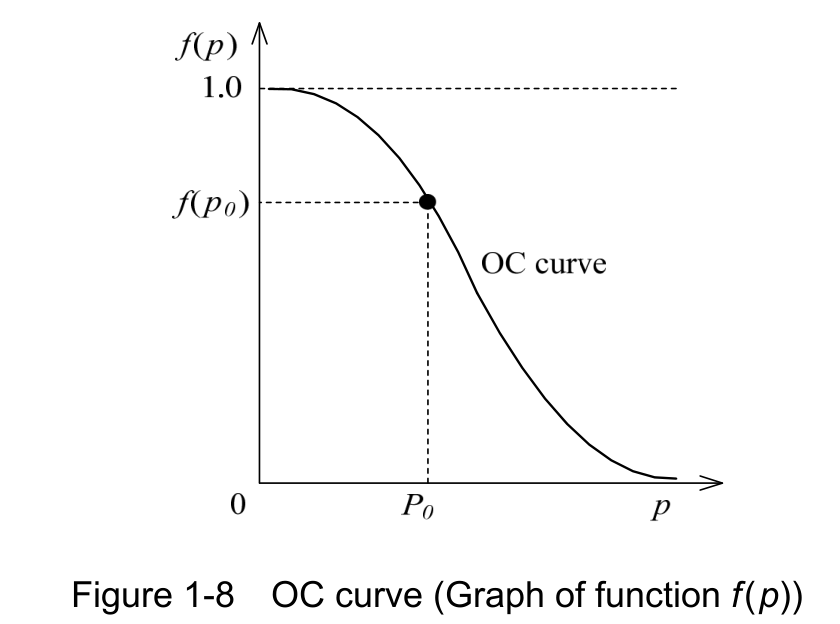
Source visual description

Original Figure 1-8, OC curve (Graph of function f(p)). The vertical axis is f(p), with 1.0 and f(p0) reference levels; the horizontal axis is p, with 0 and p0 labels. The descending OC curve and the original marked point, dotted guides and caption remain intact.

Original visual text

Figure 1-8 OC curve (Graph of function f(p))

As shown by the OC curve in Figure 1-8, when the defective rate is p0, the inspection pass rate of the population becomes f(p0). However, even if the real defective rate of the population is higher than p0, the inspection may incorrectly result in a pass. This is called consumer’s risk for its inconvenience to the product user. On the other hand, even if the real defective rate of the population is lower than p0, the inspection may result in a reject. This is called producer’s risk for its inconvenience to the producer. OC curves are also used in defective rate estimation, which estimates the defective rate from the inspection pass rate. · 2 questions

(ii) 100-percent inspection This method is to inspect each individual product. While it offers certainty as a method, its applications are limited if the cost and time that are required to inspect all products are considered.

(iii) Simulation This method is to model complex events that are difficult to actually carry out, and predict the results. In the inspection technique, inspection results are predicted through simulation before the inspection is performed, and are deemed to have passed if they

p. 76 · PDF 80

fall within a predicted range. For example, the failure rate for machinery, which is used in manufacturing products, is modeled with a failure rate curve (bathtub curve), as shown in Figure 1-9. This is used in such cases of estimating (or predicting) the defective rate of manufactured products from the failure rate of machinery.

Enlarge original visual

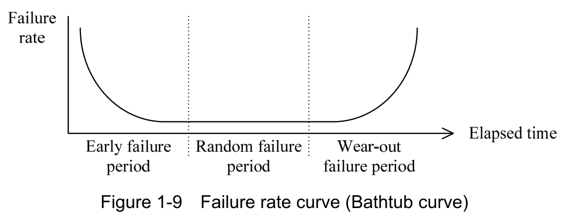
Source visual description

Original Figure 1-9, Failure rate curve (Bathtub curve). Vertical Failure rate and horizontal Elapsed time axes are retained. The curve passes through Early failure period, Random failure period and Wear-out failure period, separated by the original dotted vertical lines.

Original visual text

Figure 1-9 Failure rate curve (Bathtub curve)

(2) QFD (Quality Function Deployment)

QFD (Quality Function Deployment), which is defined by JIS Q 9025, is a methodology for using various changes and expansions in order to achieve quality goals for products. Quality function deployment is a general name for the following five deployments, and can be summarized in a deployment table in which the results of hierarchically analyzing elements are systematically displayed.

• • Quality deployment
  This is a method that converts required quality into quality characteristics (i.e., characteristics that are originally built into products, processes, or systems which is related to required quality), defines the design quality of products, and expands this to the quality of each functional component/individual component, and elements of processes.
• • Engineering deployment
  This is a method that considers whether the functions to implement design quality can be achieved with currently possible features, and identifies bottleneck technologies. The deployment by a company of its own technology is also sometimes called engineering deployment.
• • Cost deployment
  This is a method that seeks to reduce costs or identify problems in costs by allocating target costs in response to required quality or functions.
• • Reliability deployment
  This is a method that clarifies guaranteed items for reliability with respect to required

p. 77 · PDF 81

quality.

• • Job function deployment
  This is a method that hierarchically analyzes and clarifies the work that forms quality.

(3) 7 QC tools/New 7 QC tools

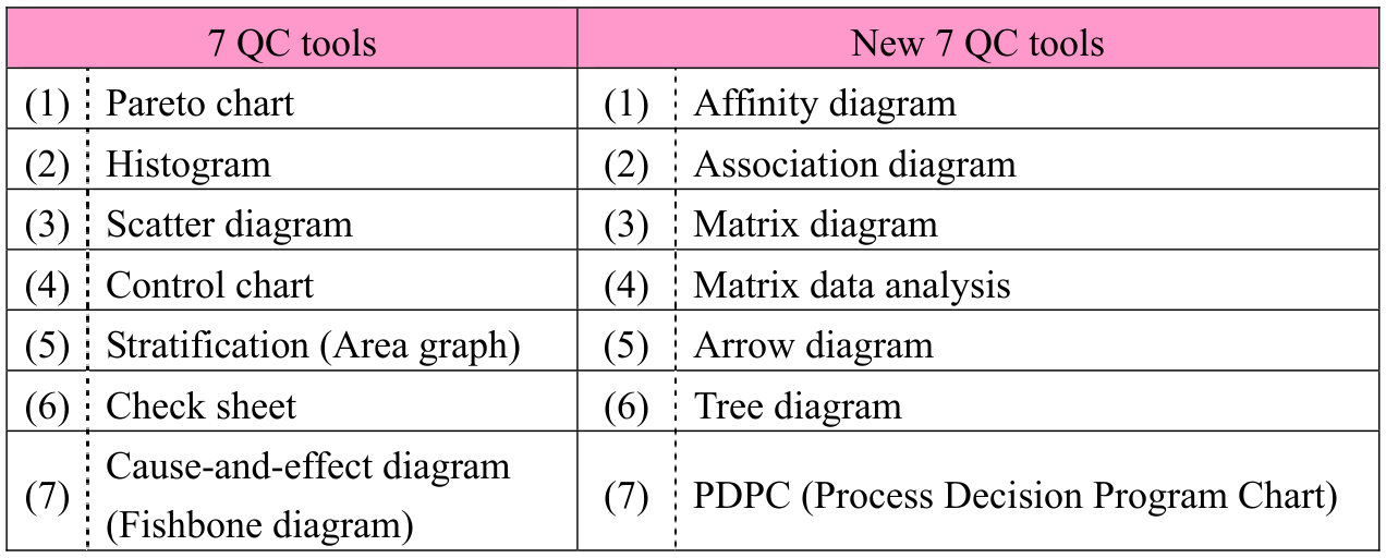
7 QC tools and new 7 QC tools are diagramming techniques that are used in quality control. The 7 QC tools have long been used primarily for manufacturing and inspection departments. On the other hand, the new 7 QC tools have been proposed as QC techniques for sales, service, and R&D departments, within TQC (Total Quality Control) which is involved in organizations in all departments and at all levels. The following are the technique (or diagram) names of the 7 QC tools and the new 7 QC tools.

7 QC tools	New 7 QC tools
(1) Pareto chart	(1) Affinity diagram
(2) Histogram	(2) Association diagram
(3) Scatter diagram	(3) Matrix diagram
(4) Control chart	(4) Matrix data analysis
(5) Stratification (Area graph)	(5) Arrow diagram
(6) Check sheet	(6) Tree diagram
(7) Cause-and-effect diagram (Fishbone diagram)	(7) PDPC (Process Decision Program Chart)

View original table · p. 77

Enlarge original table

[7 QC tools]

(1) Pareto chart This is a diagram that combines a bar graph and line graph to enable control and analysis by viewing the cumulative total percentages of the whole. Specifically, a bar graph is drawn with bars in descending orders by quantity, and the cumulative total percentage of the whole for each bar is represented with a line graph. This is used in situations including ABC analysis, which clarifies key control items.

(2) Histogram This is a diagram that allows to understand the overall characteristics or the data variability by dividing the range of data into several sections and plotting the number of data items in each section as a bar graph.

p. 78 · PDF 82

(3) Scatter diagram This is a graph that sets two corresponding types of data on the vertical and horizontal axes, after which the measured values are plotted. It enables correlation between the data sets (i.e., the presence of mutual influence) to be viewed through the degree of dispersion of points. (This is used in correlation analysis and regression analysis.) In particular, a diagram in which points on the graph are displayed as some number of groups and allows to view data characteristics, may be called a portfolio diagram. · 1 question

(4) Control chart In a control chart, a CL (Central Line) that represents normal values, a UCL (Upper Control Line) that represents the upper limit of normal values, and an LCL (Lower Control Line) that represents the lower limit of normal values are all written, and then data (i.e., mean value) is plotted as a point and each point is connected to be displayed as a line graph. When data such as the changes in product size, weight, or constituents, or the number of occurrences of defectives, differs significantly from other data, a control chart allows identification of whether the difference is caused by chance or caused by abnormality in manufacturing processes. When the plotted data falls within the range of the control lines, manufacturing processes are normal. However, when the data falls outside the range of the control lines or deviates from the norm, improvement is needed. In contrast to an X control chart on which mean values are plotted, · 1 question

there is also the R control chart on which the data range (i.e., “maximum value − minimum value”) is plotted.

(5) Stratification (Area graph) Stratification is the classification of data. For example, raw materials for a product can be classified by manufacturer, by lot, by place of production, by size, and so on. Even problems that appear complex can be made simple through classification, and it becomes easier to discover a solution. In place of stratification, area graphs may be included. An area graph is a type of line graph that makes time series analysis easy.

(6) Check sheet This is a table or diagram that is formatted in advance so as to enable understanding of a whole by collecting itemized data and confirming items through checks. (7) Cause-and-effect diagram (Fishbone diagram) This is a diagram for systematically organizing the relationships between

characteristics (or effects) and factors (or causes), in order to uncover causes.

p. 79 · PDF 83

Enlarge original visual

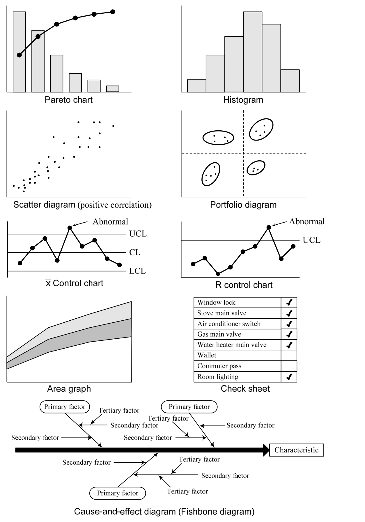
Source visual description

Original examples of the seven QC tools: Pareto chart, Histogram, Scatter diagram (positive correlation), Portfolio diagram, x-bar Control chart, R Control chart, Area graph, Check sheet, and Cause-and-effect diagram (Fishbone diagram). The original UCL, CL, LCL and Abnormal labels, check-sheet entries, characteristic box, primary/secondary/tertiary factor labels, plotted points, lines, bars and arrows remain intact.

Original visual text

[New 7 QC tools]

(1) Affinity diagram This is a diagram that, for complex and ambiguous problems, sorts items on the basis of resemblance and strength of the relevance, and then organizes and

p. 80 · PDF 84

groups problem discovery and causal relationships.

(2) Association diagram This is a diagram that organizes effects (or problem points) and causes, and causal relationships such as objectives and measures, by connecting these with arrows. It is used to clarify causal relationships for problems in which complex factors are intertwined, and to reveal clues to solutions or to solve the causes of problems.

(3) Matrix diagram This arranges problem elements (or data) in rows i.e., (horizontal axis) and columns (i.e., vertical axis), and uses symbols to represent the existence or degree of relationships at the intersections of row and column elements. It is used to clarify the relationships among data.

(4) Matrix data analysis This is an analytical method that is used when numerical data is handled in a matrix diagram. It can be used for when trends cannot be grasped from voluminous numerical data, and for discovering key items. Roughly speaking, the procedures for matrix data analysis are: arrangement of elements (or data) in a matrix; calculation of correlation coefficients; analysis of causal relationships; and display of the existence and degree of relationships at the intersections of row and column elements.

(5) Arrow diagram (Refer to p.59 for the details.)

This is a diagram that uses arrows to display the flow of each activities, on the basis of its preceding activities. It is used to find the total number of days required, or key management activities, in scheduling.

(6) Tree diagram (Logic tree) This is a diagram that seeks approaches or plans that are required to achieve objectives or goals, organizes the findings, and displays these in tree form. It is effective in uncovering the core of a problem and opening a path to a solution, while group members redraw the relation diagram with reaching consensus and overturning ideas between them. (7) PDPC (Process Decision Program Chart) This is a diagram used to predict conceivable outcomes and situations, prevent trouble, and move forward with plans in as desirable a direction as possible.

p. 81 · PDF 85

Enlarge original visual

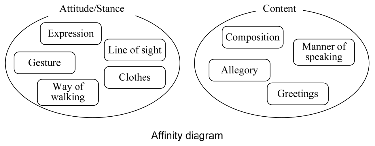
Source visual description

Original Affinity diagram. One group is Attitude/Stance, containing Expression, Line of sight, Gesture, Clothes and Way of walking. The Content group contains Composition, Manner of speaking, Allegory and Greetings. The original group ovals and caption remain together.

Original visual text

p. 82 · PDF 86

Enlarge original visual

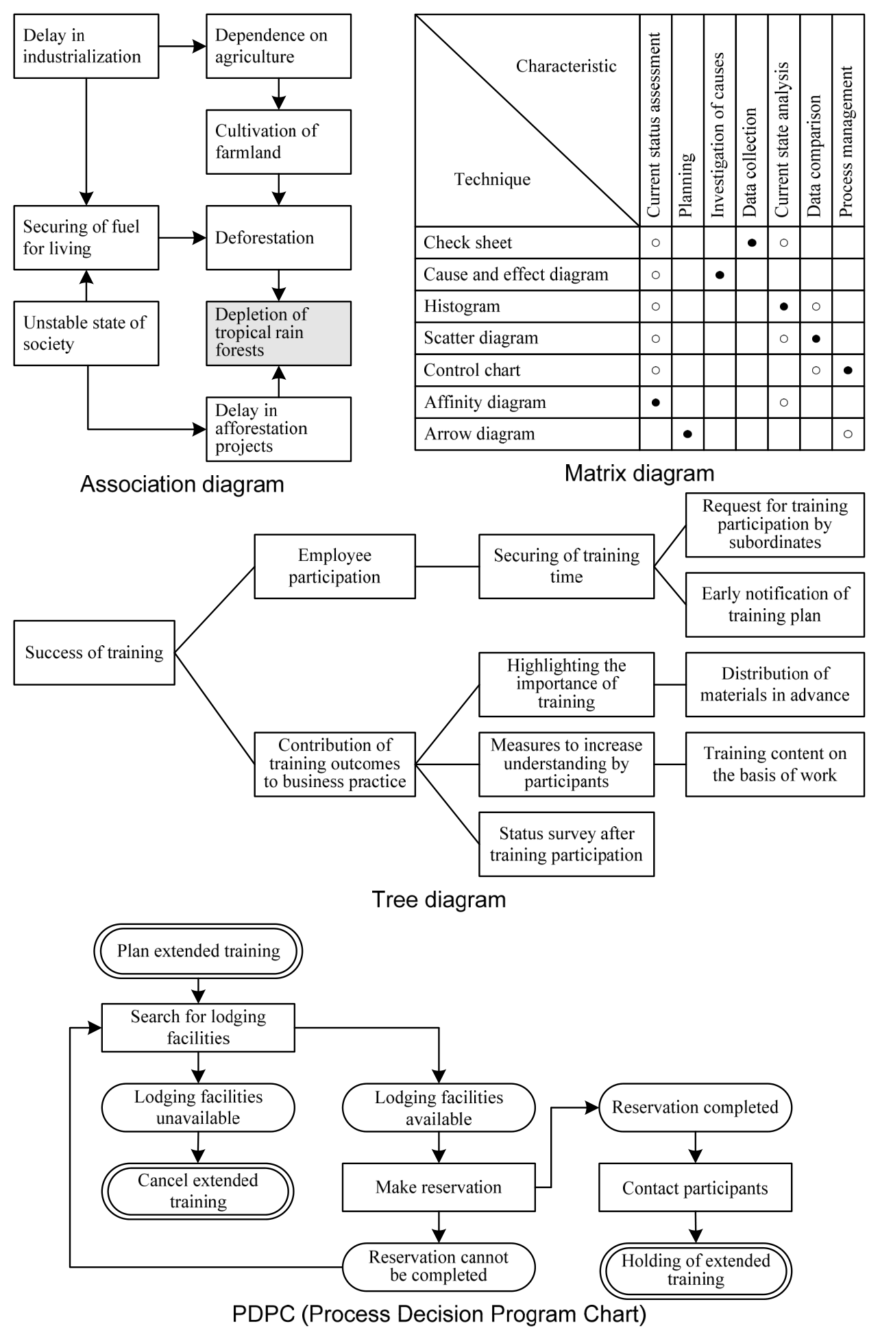
Source visual description

Original examples labeled Association diagram, Matrix diagram, Tree diagram and PDPC (Process Decision Program Chart). The association diagram retains its linked industrialization/agriculture/food/project statements. The matrix retains every row and column label, filled and hollow circle marks. The tree diagram retains the training-success branching example. The PDPC retains its extended-training planning, lodging, cancellation/reservation, participant and end-point branches. All original connectors, boxes and captions are preserved.

Original visual text