Learning toolsProgress & bookmarks
p. 49 · PDF 53
3-1-5 Numerical Analysis
Numerical analysis is a computer-aided calculation method of finding an approximate value of the complex calculation that is difficult to find an exact solution. This section explains the basic knowledge that is required for numerical analysis.
(1) Matrix
A matrix is a set of numbers that is aligned in a square or rectangular shape. The matrix A with 2 rows and 2 columns and the inverse matrix A-1 (i.e., a matrix which results in the identity matrix I when it is multiplied with A) can be formulated as shown below.

Source visual description
The first matrix has first row a, c and second row b, d. The inverse has scalar numerator 1 and denominator a d minus b c, followed by rows d, minus c and minus b, a. The product A times its inverse is I, shown with rows 1, 0 and 0, 1.
Selectable source glyphs (PDF extraction order)
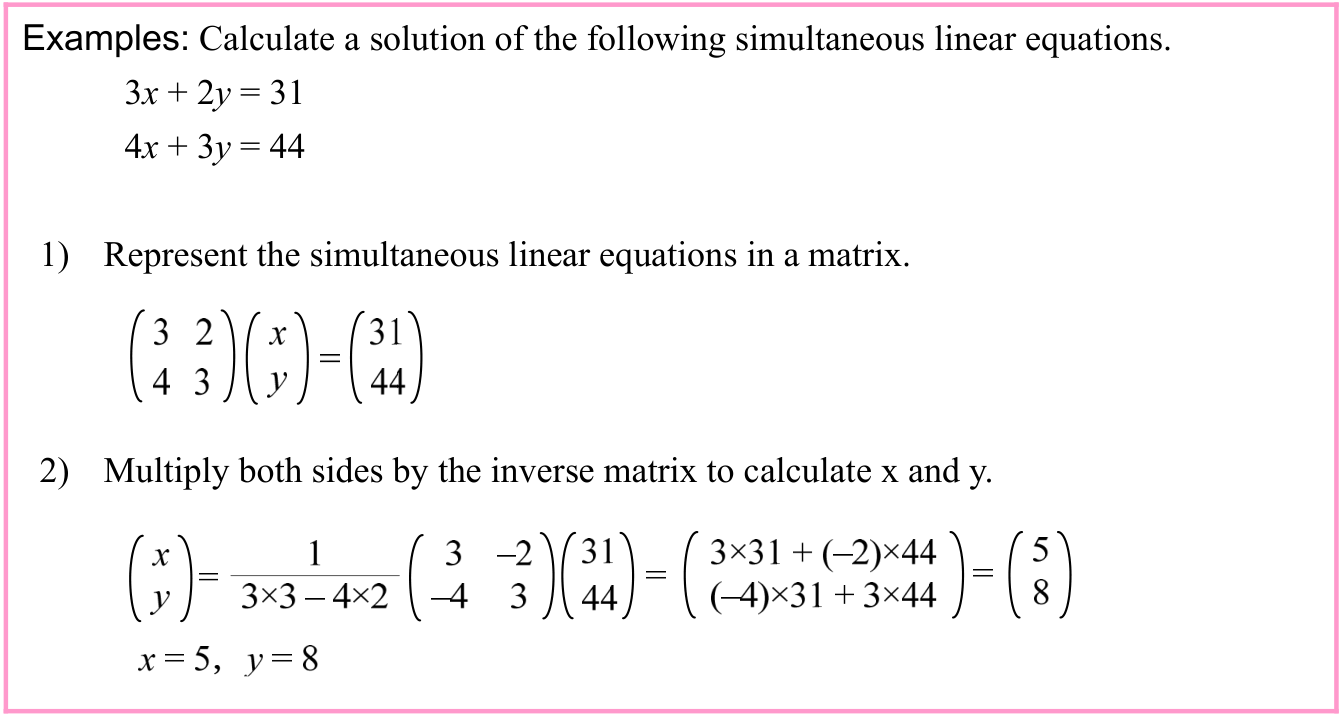
Matrices can be used to solve equations, such as simultaneous linear equations.
Source visual description
The original simultaneous equations are 3x + 2y = 31 and 4x + 3y = 44. Both source steps, matrix rows, inverse entries, products and final values x = 5, y = 8 are retained.
Selectable source glyphs (PDF extraction order)
Examples: Calculate a solution of the following simultaneous linear equations. 3x + 2y = 31 4x + 3y = 44 1) Represent the simultaneous linear equations in a matrix. 2) Multiply both sides by the inverse matrix to calculate x and y.
(2) Factorization
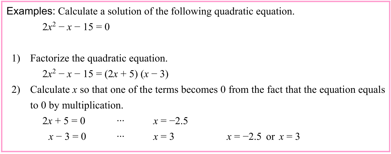
Factorization is a process which converts an integer (or integral expression) into the product of multiple integers (or the product of integral expressions). (The reverse process is called
p. 50 · PDF 54
“expansion of expression.”) Factorization is used for solutions to problems, such as higher-degree equations.
Source visual description
The original quadratic equation, its two factors, both zero-factor equations and the final alternatives minus 2.5 and 3 are transcribed in their source order.
Selectable source glyphs (PDF extraction order)
Examples: Calculate a solution of the following quadratic equation. 2x2 − x − 15 = 0 1) Factorize the quadratic equation. 2x2 − x − 15 = (2x + 5) (x − 3) 2) Calculate x so that one of the terms becomes 0 from the fact that the equation equals to 0 by multiplication. 2x + 5 = 0 ··· x = −2.5 x − 3 = 0 ··· x = 3 x = −2.5 or x = 3
(3) Logarithm

Source visual description
The original paragraph displays a = b raised to x, x = log base b of a, and the common-logarithm example log base 10 of 2 approximately 0.3010. The lower base labels and exponent positions are retained.
Selectable source glyphs (PDF extraction order)
A logarithm refers to the x in an equation, such as a = b x, and is represented as x = log b a (which is read as “x is the log base b of a”). Logarithms of base 10 are particularly called common logarithms, and also the base number 10 is often omitted (e.g., log x) (log102 ≈ 0.3010.) The following laws apply to logarithm:

Source visual description
The original Law 1, Law 2 and Law 3 rows retain their bases, exponent, division sign and printed restriction n > 0, n not equal to 1.
Selectable source glyphs (PDF extraction order)
[Law 1] log b a n = n × log b a [Law 2] log b (x × y) = log b x + log b y [Law 3] log b a = log n a ÷ log n b (n > 0, n ≠ 1)
(4) Differentiation and integration
The following is a summary of the differential and integral relationships of a function f(x).

Source visual description
The left box reads Function: x raised to n. The right reads Derivative: n times x raised to n minus 1. The upper arrow points right and is labelled Differentiation, with f(x) and f-prime(x). The lower arrow points left and is labelled Integration, with the integral of f(x) dx and f(x).
Selectable source glyphs (PDF extraction order)
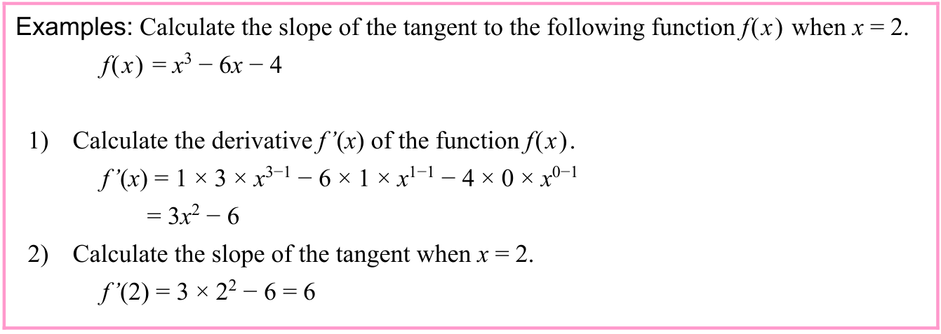
Differentiation is used for such tasks as calculating the slope of a tangent. In order to use Newton’s method which is used to calculate a solution of higher-degree equation f(x) = 0, since the tangent to the function f(x) must be calculated, the function f(x) must be differentiable.
p. 51 · PDF 55
Source visual description
The original example evaluates the derivative of x cubed minus 6x minus 4 at x = 2. The expanded source differentiation row includes its printed zero-coefficient term and exponent zero minus one; no source term is omitted.
Selectable source glyphs (PDF extraction order)
Examples: Calculate the slope of the tangent to the following function f(x) when x = 2. f(x) = x3 − 6x − 4 1) Calculate the derivative f’(x) of the function f(x). f’(x) = 1 × 3 × x3−1 − 6 × 1 × x1−1 − 4 × 0 × x0−1 = 3x2 − 6 2) Calculate the slope of the tangent when x = 2. f’(2) = 3 × 22 − 6 = 6
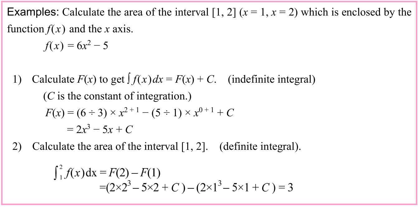
Integration is used for tasks, such as finding the area within an interval that is enclosed by a curve. The integral with the constant of integration is called an indefinite integral. An integral for which the interval of integration is defined is called a definite integral.
Source visual description
The source function is 6x squared minus 5. The original indefinite integral retains the constant C. The definite-integral bounds are 1 below and 2 above the integral sign. The complete substitution and source result 3 remain intact.
Selectable source glyphs (PDF extraction order)
Examples: Calculate the area of the interval [1, 2] (x = 1, x = 2) which is enclosed by the function f(x) and the x axis. f(x) = 6x2 − 5 1) Calculate F(x) to get ∫ f(x)dx = F(x) + C. (indefinite integral) (C is the constant of integration.) F(x) = (6 ÷ 3) × x2 + 1 − (5 ÷ 1) × x0 + 1 + C = 2x3 − 5x + C 2) Calculate the area of the interval [1, 2]. (definite integral).
(5) Bisection method
The bisection method is a method to calculate an approximate solution for higher-degree equation f(x) = 0. This method works by repeating the process of dividing the range of possible solutions in half to approach the actual solution. In compared with Newton’s method, which utilizes the tangent of f(x) to calculate the approximate solution, this method is slower to converge at the solution.
p. 52 · PDF 56
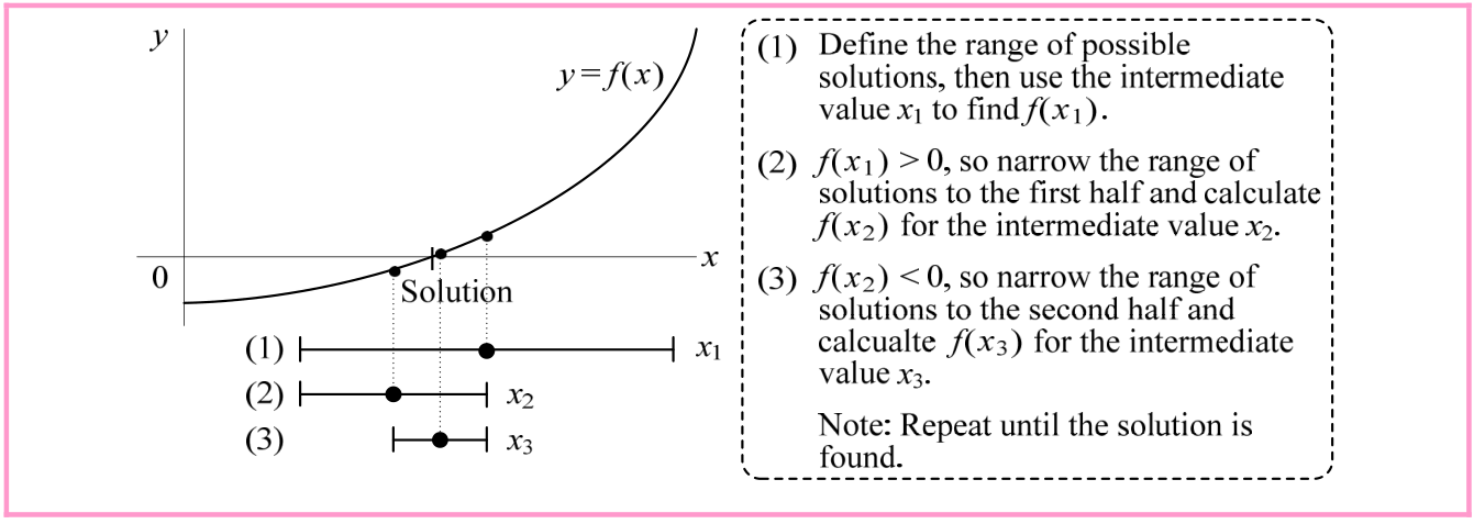
Source visual description
The original rising curve is labelled y = f(x), with axes x and y and a point labelled Solution. The three numbered interval rows mark x1, x2 and x3 with lower indices. The source callout states f(x1) > 0 and f(x2) < 0 in its second and third steps, and repeats until the solution is found.
Selectable source glyphs (PDF extraction order)
It is necessary to be aware of the following types of error that can occur when bisection method calculations are performed. There are two methods of representing error: absolute error, which represents the degree of error directly, and relative error, which represents the error as a percentage (i.e., ratio) to the true value.
- • Rounding Error
When a computer has to represent a real number with a limited number of digits, error is introduced by rounding off, rounding up, or truncating the value to the digits that are less than the least digit. - • Truncation Error
This error is caused by truncating after a limited number of passes on the basis of specified conditions (e.g., convergence value, repeat count) when calculations could be repeated infinitely.
(6) Interpolation method
Interpolation method is a method to find the function value f(x) in regards to an unknown variable by deriving the polynomial f(x) from the relationship between known discrete variables.
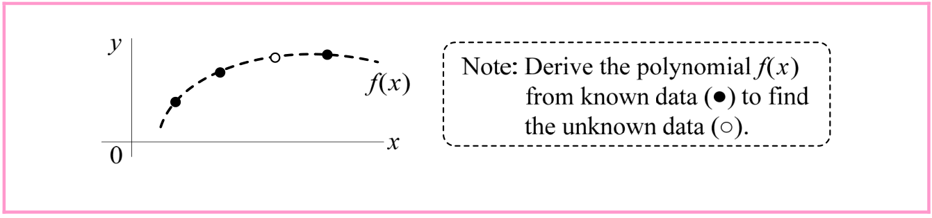
Source visual description
The graph has axes x and y, 0, and a dashed curve labelled f(x). Filled points mark known data and the open point marks unknown data. The callout says to derive the polynomial f(x) from known data to find the unknown data.
Selectable source glyphs (PDF extraction order)
Common interpolation methods are Lagrange interpolation and spline interpolation. Interpolation is used in fields such as CG (computer graphics) to draw curves. The concepts,
p. 53 · PDF 57
such as trapezoid rule and Simpson’s method, are also types of interpolation, which are used to find the area that is enclosed by a curve and the x axis.
Section progress
Original chapter exercises
Original chapter exercises →New FE Textbook Vol.2 · First Edition, April 2015