Highlighted text? Practice this concept. Highlighted passages and figures open related questions.
Practice related questions (2)Progress & bookmarks
Current section
3-1-4 Statistics
p. 43
Practice this section 2 linked exam questions with default filters
Progress
Not marked complete
Related questions in this lesson 3
Standard normal distribution1Linear equations for estimating demand1Correlation analysis1p. 43 · PDF 47
3-1-4 Statistics
Statistics is a mathematical technique that is used to find patterns in large sets of data. In natural, economic, and social phenomena, each set of data may seem random at first glance, but in some cases there may be a specific trend or pattern. For example, the probability (i.e., mathematical probability) of rolling a 1 in a single dice throw is 1/6. However, if the dice is rolled 10 times, it may not be possible to get a single 1 in real. However, the more times the dice is rolled, the closer the probability will approach 1/6. (This is called statistical probability or empirical probability.) Statistics is a method of finding patterns through repeated measurements and/or observations. In statistics, the entire set of target data is called the population, and a survey of this data is called a complete survey. A portion of a population is called a sample, and sampling data from a population for surveying is called a sample survey. Generally, statistics is used to determine certain characteristics (e.g., trends, patterns) from a sample survey and to estimate
p. 44 · PDF 48
the characteristics of a population.
(1) Frequency distribution
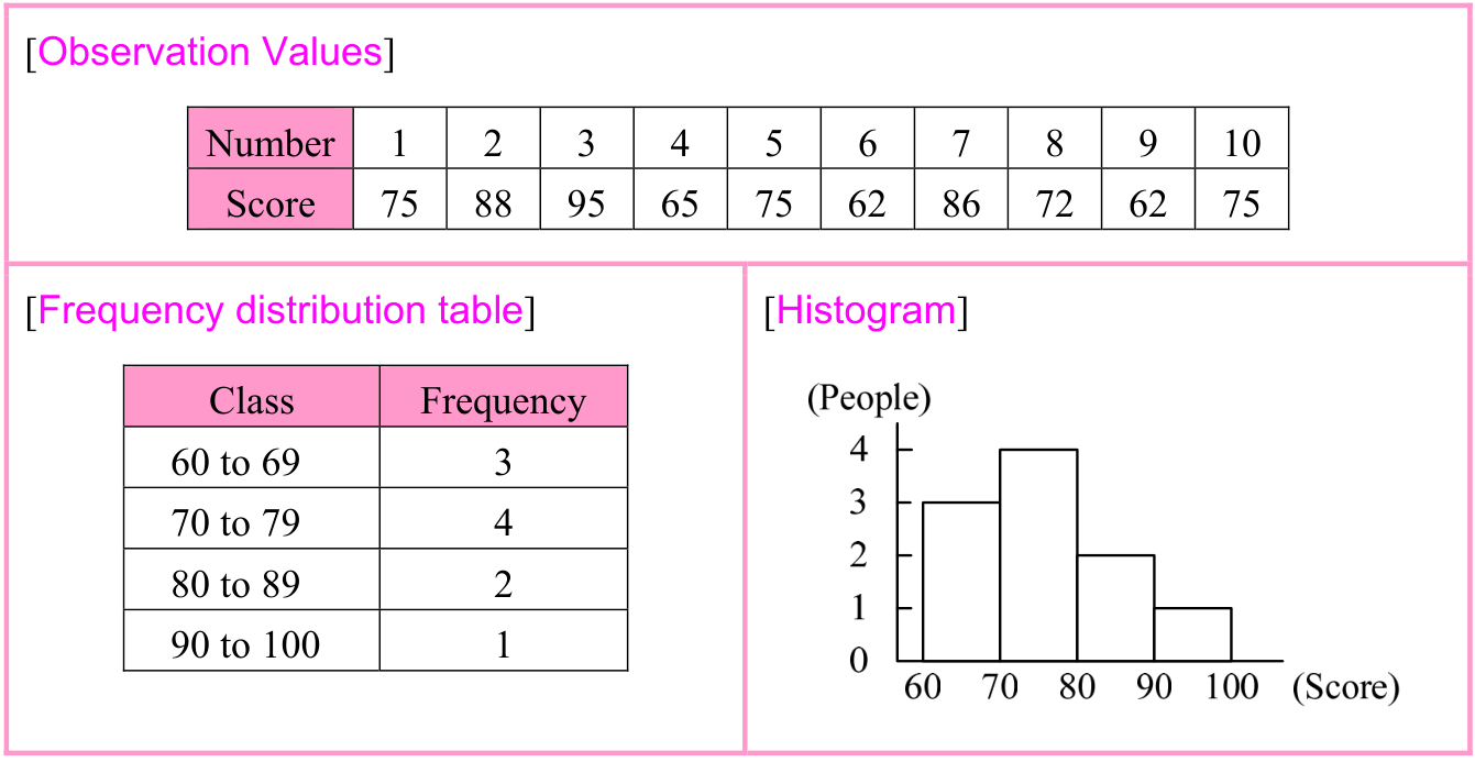
Frequency distribution refers to the distribution status of the frequency (i.e., the number of observation values in a set of measurement data) between intervals. Frequency distributions are often represented in a frequency distribution table or a histogram.
Source visual description
The observation table gives Number 1 through 10 and Score 75, 88, 95, 65, 75, 62, 86, 72, 62, 75. The frequency table columns are Class and Frequency: 60 to 69 has 3; 70 to 79 has 4; 80 to 89 has 2; 90 to 100 has 1. The histogram uses vertical People labels 0, 1, 2, 3, 4 and horizontal Score labels 60, 70, 80, 90, 100. All three original panels are kept together.
Selectable source glyphs (PDF extraction order)
[Observation Values] Number 1 2 3 4 5 6 7 8 9 10 Score 75 88 95 65 75 62 86 72 62 75 [Frequency distribution table] [Histogram] Class Frequency 60 to 69 3 70 to 79 4 80 to 89 2 90 to 100 1
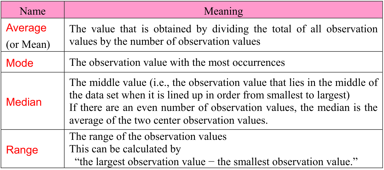
(i) Representative value This is a value that represents a characteristic of the observation values (e.g., overall trend, pattern). The following are types of representative values:
| Name | Meaning |
|---|---|
| Average (or Mean) | The value that is obtained by dividing the total of all observation values by the number of observation values |
| Mode | The observation value with the most occurrences |
| Median | The middle value (i.e., the observation value that lies in the middle of the data set when it is lined up in order from smallest to largest) If there are an even number of observation values, the median is the average of the two center observation values. |
| Range | The range of the observation values This can be calculated by “the largest observation value − the smallest observation value.” |
p. 45 · PDF 49
Source visual description
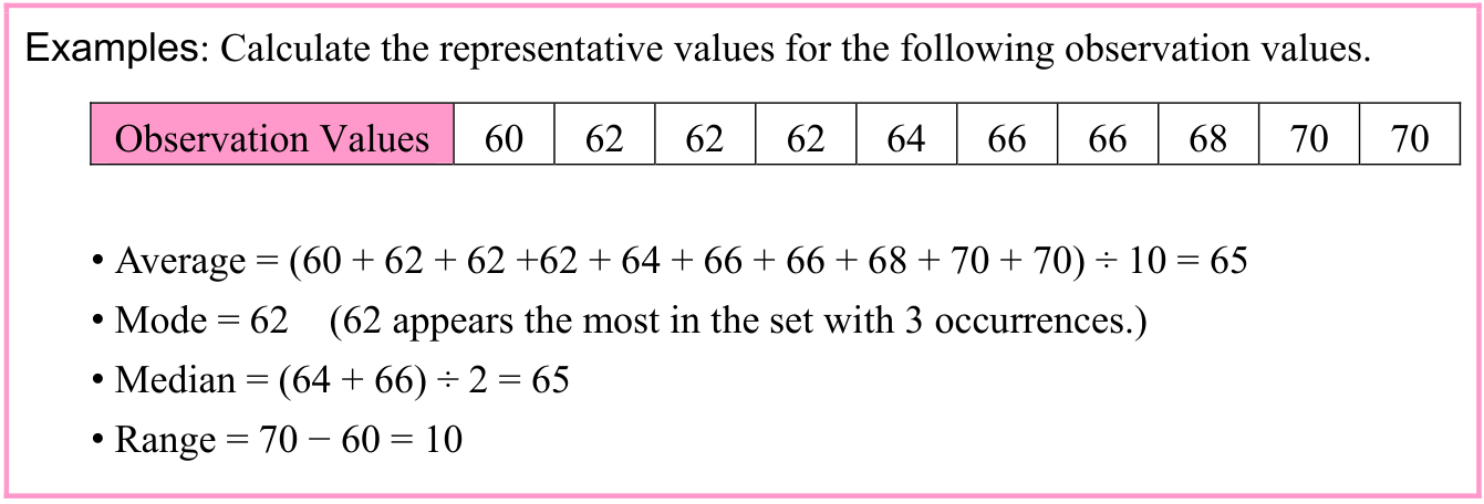
The observation values are 60, 62, 62, 62, 64, 66, 66, 68, 70, 70. The original results are Average 65, Mode 62 with 3 occurrences, Median 65 and Range 10. The printed division signs and source minus character are retained.
Selectable source glyphs (PDF extraction order)
Examples: Calculate the representative values for the following observation values. Observation Values 60 62 62 62 64 66 66 68 70 70 • Average = (60 + 62 + 62 +62 + 64 + 66 + 66 + 68 + 70 + 70) ÷ 10 = 65 • Mode = 62 (62 appears the most in the set with 3 occurrences.) • Median = (64 + 66) ÷ 2 = 65 • Range = 70 − 60 = 10
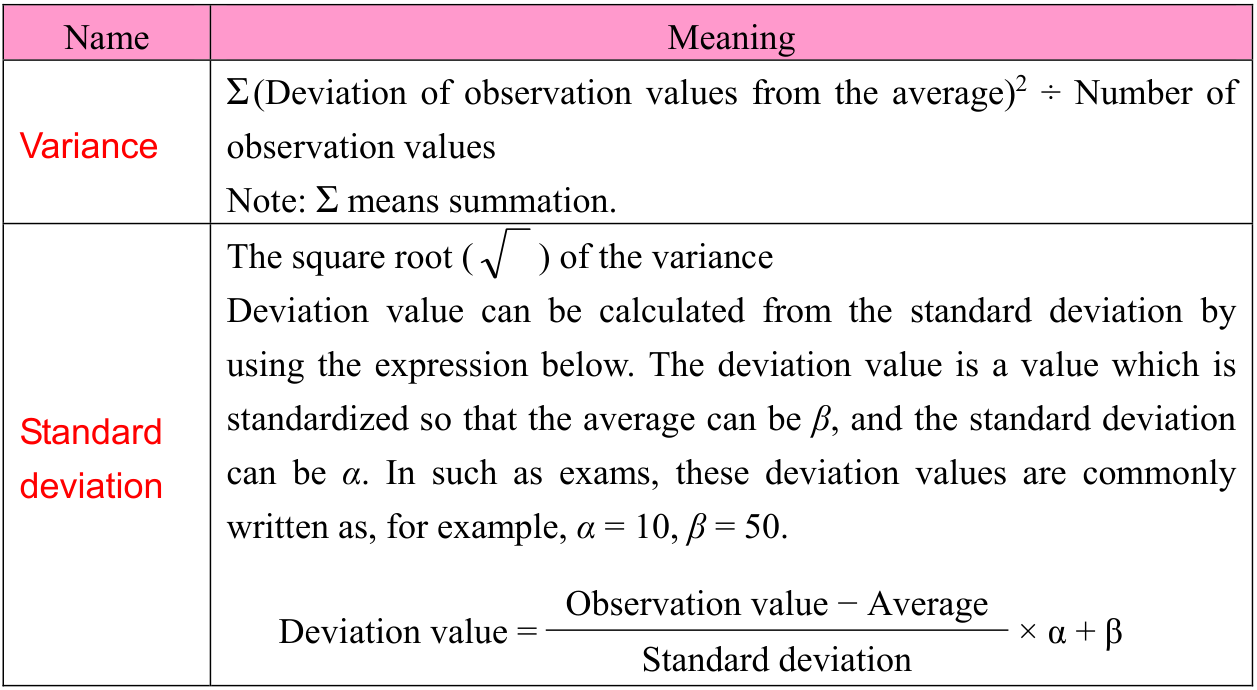
(ii) Dispersion This is a value that represents the degree of scatter (i.e., degree of dispersion) in a set of observation values. The types of dispersion are listed below. For all of these types, the higher the number, the higher the scatter, and the lower the number, the closer all observation values are to the average.
Source visual description
The rows are Variance and Standard deviation. Variance is the printed capital-Sigma expression for squared deviations divided by the number of observation values; its note states Sigma means summation. Standard deviation is the square root of variance. The original deviation-value paragraph uses average beta and standard deviation alpha, with example alpha = 10, beta = 50. Its fraction has Observation value minus Average above Standard deviation, then times alpha plus beta.
Selectable source glyphs (PDF extraction order)
Name Meaning Σ(Deviation of observation values from the average)2 ÷ Number of Variance observation values Note: Σ means summation. The square root ( ) of the variance Deviation value can be calculated from the standard deviation by using the expression below. The deviation value is a value which is standardized so that the average can be β, and the standard deviation Standard can be α. In such as exams, these deviation values are commonly deviation written as, for example, α = 10, β = 50. Deviation value = Observation value − Average × α + β Standard deviation
p. 46 · PDF 50
Source visual description
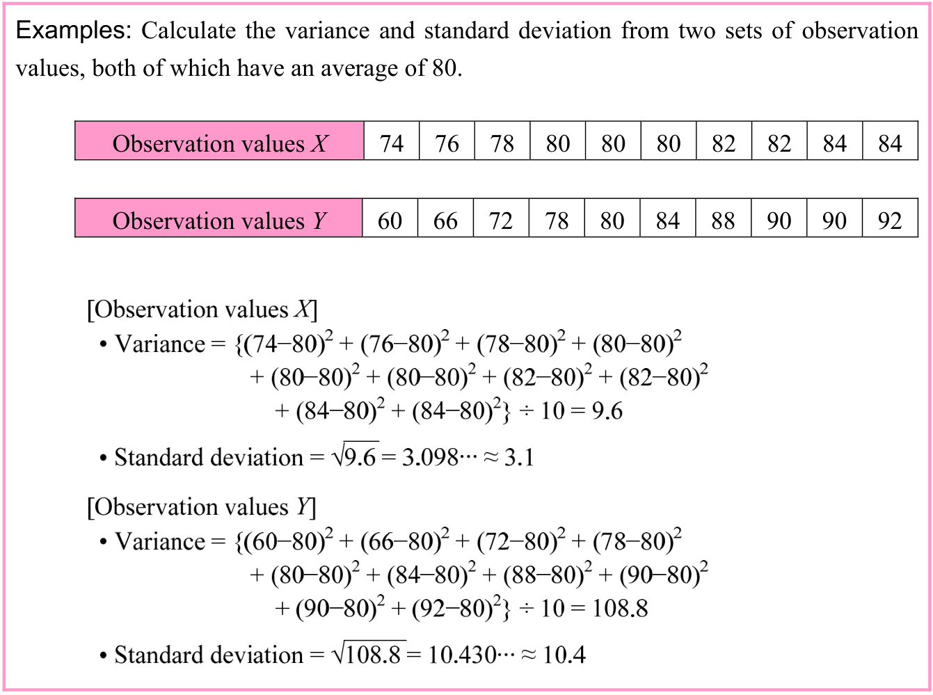
The X observations are 74, 76, 78, 80, 80, 80, 82, 82, 84, 84. The Y observation row is 60, 66, 72, 78, 80, 84, 88, 90, 90, 92. The original wording states an average of 80 for both. Each original calculation and displayed result is transcribed below in its printed order.
Selectable source glyphs (PDF extraction order)
Examples: Calculate the variance and standard deviation from two sets of observation values, both of which have an average of 80. Observation values X 74 76 78 80 80 80 82 82 84 84 Observation values Y 60 66 72 78 80 84 88 90 90 92
(2) Correlation
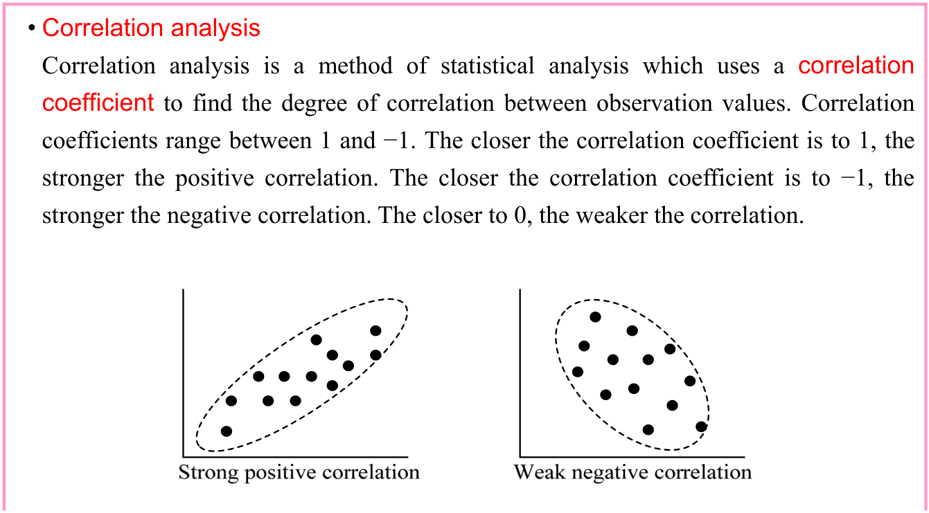
Correlation is a relationship between two variates in which changes in one variate cause changes in the other. The correlation between two sets of observation values is generally analyzed by using a scatter diagram.
Source visual description
The original correlation-analysis box continues onto the next page. It states coefficients from 1 to -1 and describes the direction and strength. The left scatter plot is captioned Strong positive correlation. The right is captioned Weak negative correlation. The source captions are retained unchanged.
Selectable source glyphs (PDF extraction order)
• Correlation analysis Correlation analysis is a method of statistical analysis which uses a correlation coefficient to find the degree of correlation between observation values. Correlation coefficients range between 1 and −1. The closer the correlation coefficient is to 1, the stronger the positive correlation. The closer the correlation coefficient is to −1, the stronger the negative correlation. The closer to 0, the weaker the correlation.
p. 47 · PDF 51
Source visual description
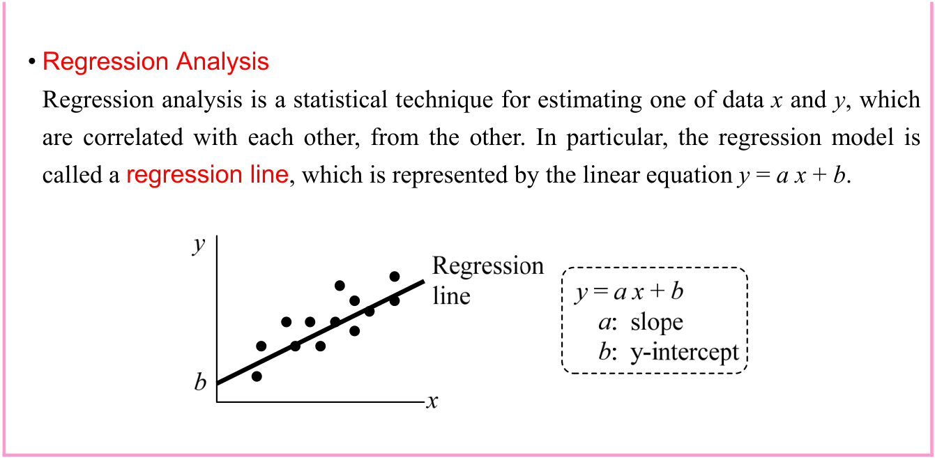
The continued box contains the original Regression Analysis paragraph and graph. The line is labelled Regression line. The axes are x and y, the intercept is b, and the callout gives y = a x + b, a: slope, b: y-intercept.
Selectable source glyphs (PDF extraction order)
• Regression Analysis Regression analysis is a statistical technique for estimating one of data x and y, which are correlated with each other, from the other. In particular, the regression model is called a regression line, which is represented by the linear equation y = a x + b.
(3) Probability distribution
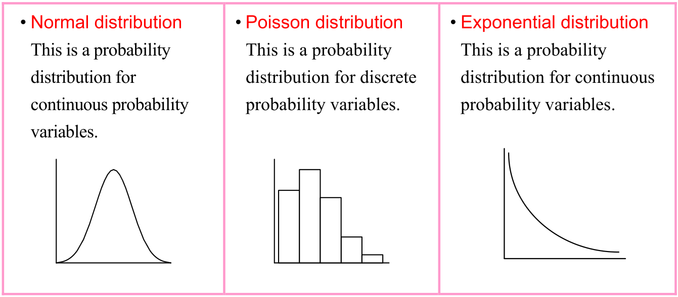
Probability distribution is the distribution status of a variable x, which has a set probability to be a certain value on the basis of the results of the trials. There are two types of probability variables: discrete probability variables which have scattered values, and continuous probability variables which must be within a continuous range. The following are the three most common types of probability distribution:
Source visual description
The original panels are Normal distribution, Poisson distribution and Exponential distribution. Their source descriptions identify continuous, discrete and continuous probability variables respectively. The original drawings are a bell curve, bars and a decreasing curve. No distribution equation has been added.
Selectable source glyphs (PDF extraction order)
• Normal distribution • Poisson distribution • Exponential distribution This is a probability This is a probability This is a probability distribution for distribution for discrete distribution for continuous continuous probability probability variables. probability variables. variables.
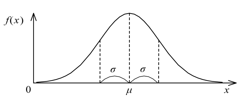
For continuous probability variables, the most commonly used probability distribution is the normal distribution. Normal distributions are written as N(μ, σ2), where N is the normal distribution, μ is the average, and σ2 is the variance. (σ is the standard deviation.) Under a normal distribution, probability characteristics are determined by the average μ and the deviation σ2, and the graph of this type of distribution is a bilaterally symmetric bell curve around the average μ.
p. 48 · PDF 52
Source visual description
The original graph has vertical f(x), horizontal x and a marked 0. The center is mu. Two sigma-marked intervals extend to either side of mu, with dashed vertical lines. All original labels and the curve are retained.
Selectable source glyphs (PDF extraction order)
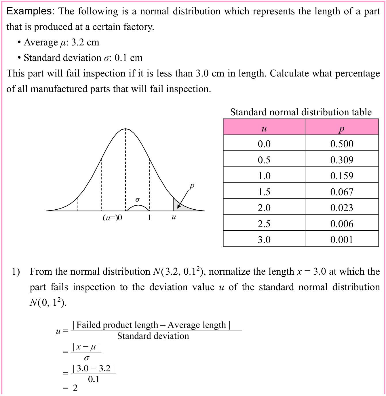
When the average or deviation of a population is estimated or determined, it is complicated to use the probability variable x as-is in those calculations. It is often easier to find the deviation value u, which is standardized to ensure that the probability variable x has an average of 0 and a standard deviation of 1, and utilize the value of u that follows a standard normal distribution N(0, 12) to find the probabilities from a standard normal distribution table.
Source visual description
The original part-length example gives average mu 3.2 cm and standard deviation sigma 0.1 cm, rejecting lengths less than 3.0 cm. The source graph is labelled u and p. The standard normal distribution table gives (u,p): (0.0,0.500), (0.5,0.309), (1.0,0.159), (1.5,0.067), (2.0,0.023), (2.5,0.006), (3.0,0.001). Absolute-value bars enclose each numerator of the original normalization calculation. The example continues on the next page.
Selectable source glyphs (PDF extraction order)
Examples: The following is a normal distribution which represents the length of a part that is produced at a certain factory. • Average μ: 3.2 cm • Standard deviation σ: 0.1 cm This part will fail inspection if it is less than 3.0 cm in length. Calculate what percentage of all manufactured parts that will fail inspection. Standard normal distribution table u p 0.0 0.500 0.5 0.309 1.0 0.159 1.5 0.067 2.0 0.023 2.5 0.006 3.0 0.001 1) From the normal distribution N(3.2, 0.12), normalize the length x = 3.0 at which the part fails inspection to the deviation value u of the standard normal distribution N(0, 12).
p. 49 · PDF 53

Source visual description
The original continuation selects p = 0.023 at u = 2.0 and concludes 2.3% of products fails inspection. Original wording is retained.
Selectable source glyphs (PDF extraction order)
2) Find the probability p where u = 2.0 from the standard normal distribution table. p = 0.023 => 2.3% of products fails inspection.
Section progress
Original chapter exercises
Original chapter exercises →New FE Textbook Vol.2 · First Edition, April 2015