Highlighted text? Practice this concept. Highlighted passages and figures open related questions.
Practice related questions (7)Progress & bookmarks
Current section
3-2 OR (Operations Research)
p. 57
Practice this section 7 linked exam questions with default filters
Progress
Not marked complete
Related questions in this lesson 15
Linear programming6Earliest node time2Latest node time1Linear-programming constraints4Economic order quantity1Maxi-min principle1Forecasting from past trends2Critical paths and zero slack3p. 57 · PDF 61
3 - 2 OR (Operations Research)
OR (Operations Research) refers to the use of statistical science technology or statistical methods to find the optimal solutions to problems that are related to system operations planning and management in order to aid in the management decision making process.
3-2-1 Linear Programming
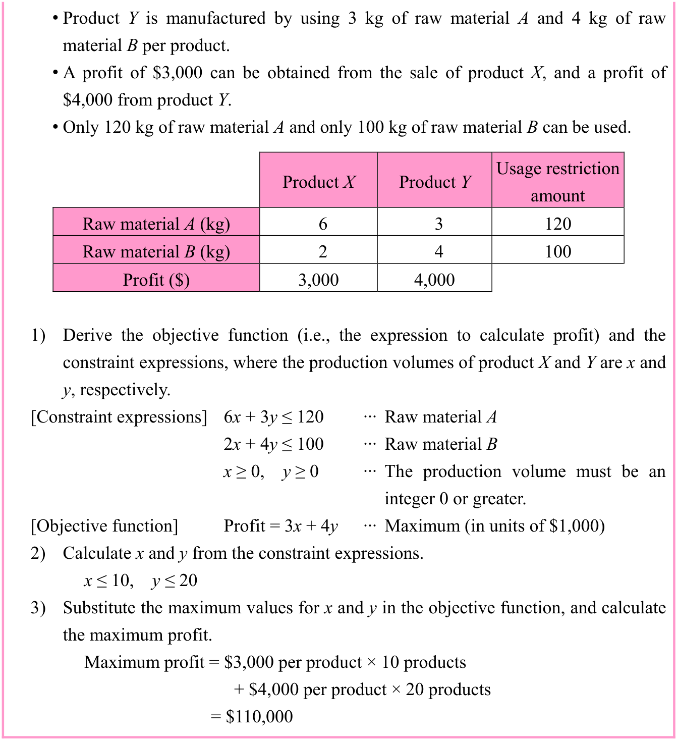
Examples: Calculate the maximum profit from the following constraints for when products X and Y are manufactured and sold by using raw materials A and B.
[Constraints]
- • Product X is manufactured by using 6 kg of raw material A and 2 kg of raw
material B per product.
p. 58 · PDF 62
Source visual description
Original source visual. Selectable source labels and wording: • Product Y is manufactured by using 3 kg of raw material A and 4 kg of raw material B per product. • A profit of $3,000 can be obtained from the sale of product X, and a profit of $4,000 from product Y. • Only 120 kg of raw material A and only 100 kg of raw material B can be used. Usage restriction Product X Product Y amount Raw material A (kg) 6 3 120 Raw material B (kg) 2 4 100 Profit ($) 3,000 4,000 1) Derive the objective function (i.e., the expression to calculate profit) and the constraint expressions, where the production volumes of product X and Y are x and y, respectively. [Constraint expressions] 6x + 3y ≤ 120 ··· Raw material A 2x + 4y ≤ 100 ··· Raw material B x ≥ 0, y ≥ 0 ··· The production volume must be an integer 0 or greater. [Objective function] Profit = 3x + 4y ··· Maximum (in units of $1,000) 2) Calculate x and y from the constraint expressions. x ≤ 10, y ≤ 20 3) Substitute the maximum values for x and y in the objective function, and calculate the maximum profit. Maximum profit = $3,000 per product × 10 products + $4,000 per product × 20 products = $110,000
Original visual text
• Product Y is manufactured by using 3 kg of raw material A and 4 kg of raw material B per product. • A profit of $3,000 can be obtained from the sale of product X, and a profit of $4,000 from product Y. • Only 120 kg of raw material A and only 100 kg of raw material B can be used. Usage restriction Product X Product Y amount Raw material A (kg) 6 3 120 Raw material B (kg) 2 4 100 Profit ($) 3,000 4,000 1) Derive the objective function (i.e., the expression to calculate profit) and the constraint expressions, where the production volumes of product X and Y are x and y, respectively. [Constraint expressions] 6x + 3y ≤ 120 ··· Raw material A 2x + 4y ≤ 100 ··· Raw material B x ≥ 0, y ≥ 0 ··· The production volume must be an integer 0 or greater. [Objective function] Profit = 3x + 4y ··· Maximum (in units of $1,000) 2) Calculate x and y from the constraint expressions. x ≤ 10, y ≤ 20 3) Substitute the maximum values for x and y in the objective function, and calculate the maximum profit. Maximum profit = $3,000 per product × 10 products + $4,000 per product × 20 products = $110,000
3-2-2 Scheduling
Scheduling is the act of creating a schedule for activities or other tasks. There are some scheduling methods, such as PERT (Program Evaluation and Review Technique) and CPM (Critical Path Method). With PERT, a plan is made for estimating an activity period. With CPM, a plan is made in consideration of shortening the schedule with a minimum cost. Sometimes, it can be difficult to distinguish between PERT and CPM, because it is sometimes written as PERT/CPM or PERT/COST which also includes costs into PERT.
p. 59 · PDF 63
[PERT characteristics]
- • Can be used for large-scale, complex projects.
- • Enables the calculation of the total number of days (i.e., minimum required work
period) to complete the project. - • Establishes a clear order of activities, which enables the understanding of a vital
point for management. - • Enables the calculation of the number of extra margin days for an activity.
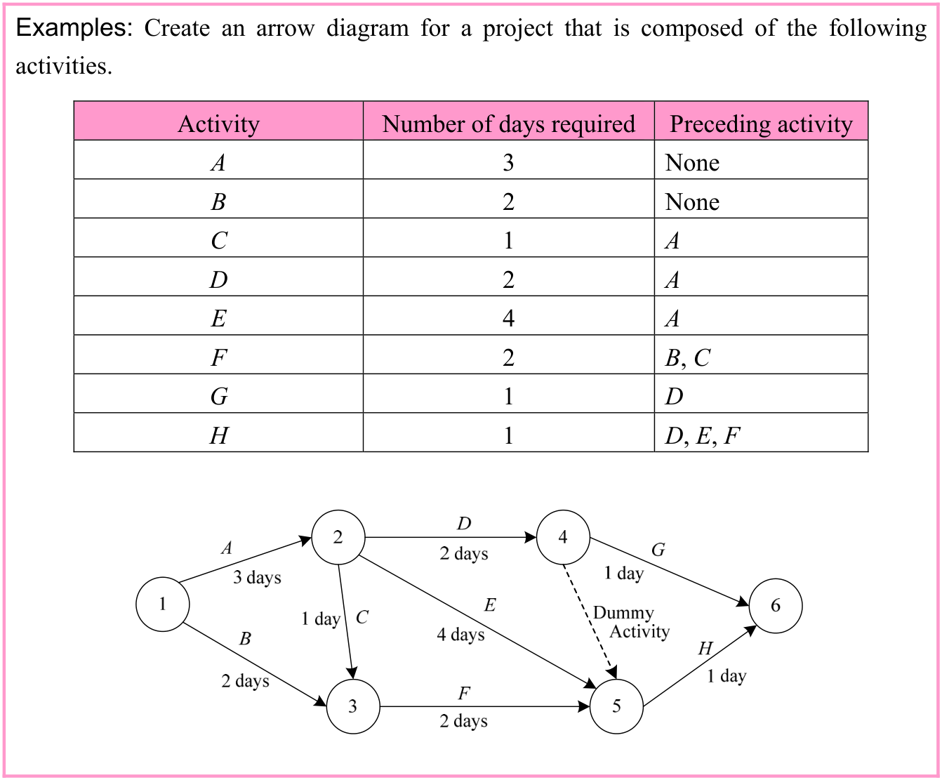
(1) Arrow diagrams
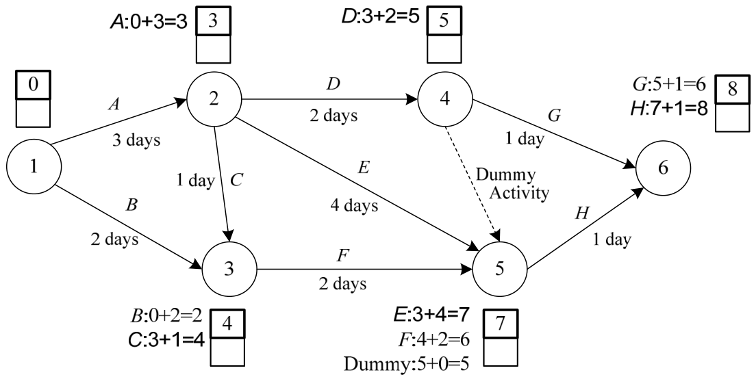
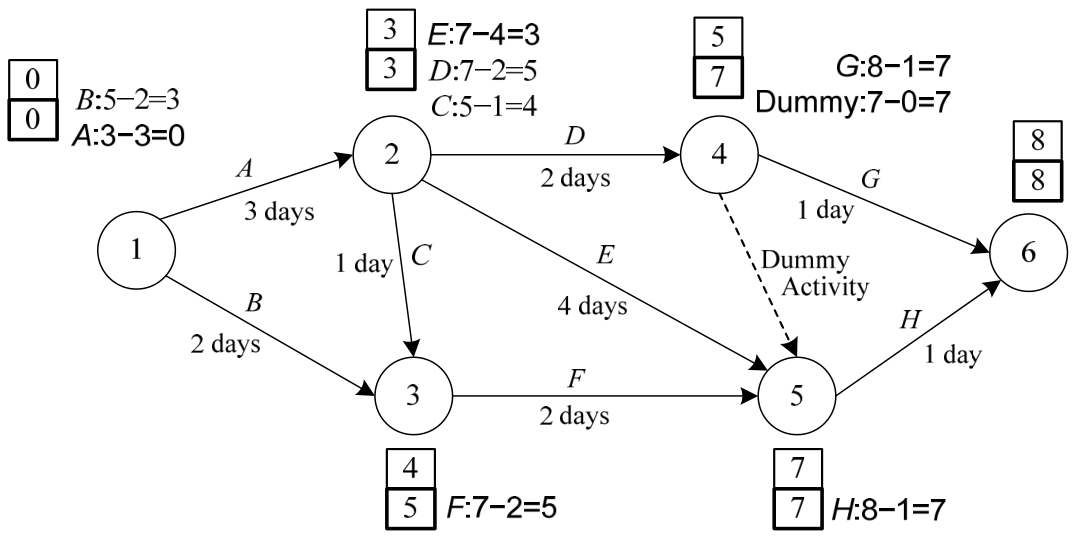
An arrow diagram is a chart which depicts the flow of each activity for a project on the basis of the preceding activity. Nodes (i.e., circles) are placed at both ends of each arrow, and the number is assigned to each node. In addition, the activity name is written above each arrow, and the number of required days below the arrow. An arrow diagram is often used in PERT, so it is sometimes called a PERT chart. It is also used in CPM and other scheduling methods.
Source visual description
Original source visual. Selectable source labels and wording: Examples: Create an arrow diagram for a project that is composed of the following activities. Activity Number of days required Preceding activity A 3 None B 2 None C 1 A D 2 A E 4 A F 2 B, C G 1 D H 1 D, E, F
Original visual text
Examples: Create an arrow diagram for a project that is composed of the following activities. Activity Number of days required Preceding activity A 3 None B 2 None C 1 A D 2 A E 4 A F 2 B, C G 1 D H 1 D, E, F
p. 60 · PDF 64
Source visual description
Original arrow diagram illustrating earliest node time. It retains numbered nodes 1 through 6, activities A through H, dummy-activity arrows, activity durations and the original forward-pass node calculations and boxed results.
Original visual text
p. 61 · PDF 65
Source visual description
Original arrow diagram illustrating latest node time. It retains nodes 1 through 6, activities, durations, dummy activities, backward-pass expressions and paired original node-time boxes.
Original visual text
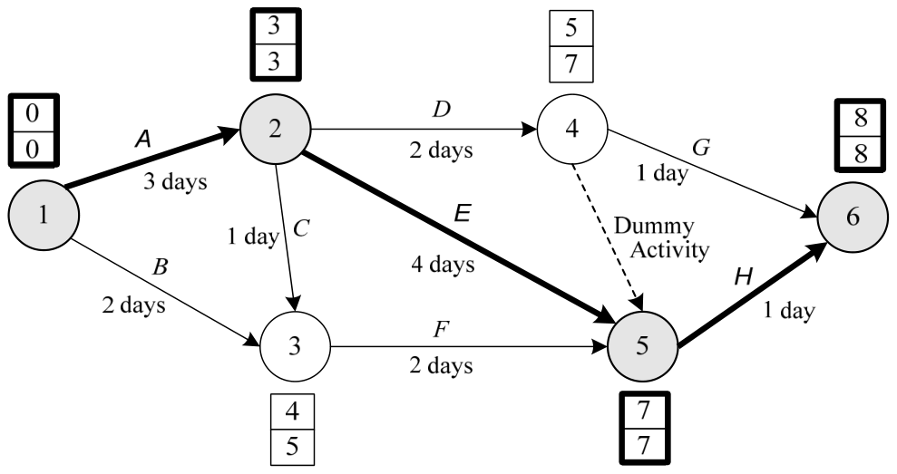
Source visual description
Original critical-path diagram. Thick arrows follow nodes 1, 2, 5 and 6 through activities A, E and H. The other activities, dummy activities, durations and each pair of node-time boxes remain visible.
Original visual text
To shorten the overall work schedule, one way is to reduce the number of days for any of the activities along a critical path. The following are different methods to shorten a work schedule.
- • Crushing
Crushing is a method in which additional staff members or cost is used to shorten the work schedule. - • Fast-tracking
Fast-tracking is a method of shortening a work schedule by breaking down specific activities into smaller parts and performing them in parallel or by
p. 62 · PDF 66
performing the next process before the completion of a preceding process.
(2) Gantt charts
A Gantt chart is a type of chart that is used to perform schedule management. For each activity, the planed activity period is written along with the actual activity period above and below, with a bar that is drawn to represent the length of an activity. This type of chart makes it easy to see the progress of an activity, but cannot be used to see the time sequence of activities.
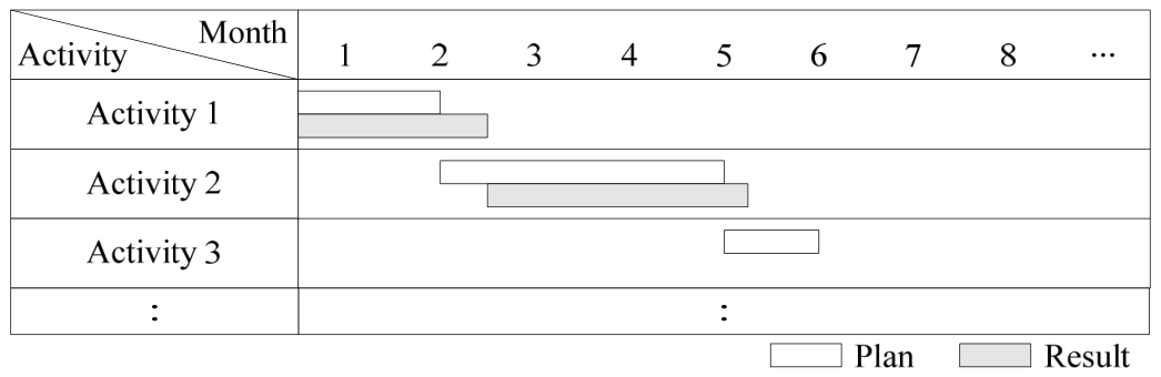
Source visual description
Original Gantt chart: rows Activity 1 through Activity 3, columns Month 1 through 8 and continuation dots. The source legend distinguishes Plan from Result; the bars and original row lengths remain intact.
Original visual text
3-2-3 Inventory Problems
An inventory problem refers to the issue of how to efficiently manage the inventory of products which are stored in a warehouse. It is important to prevent the out of stock which causes opportunity loss, and also to ensure not to have surplus stock in order to prevent increased costs.
(1) Inventory control
Inventory control is performed to manage inventory with the minimum cost, with preventing to be out of stock or surplus stock. The following terminology is used in relation to inventory control.
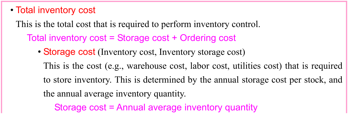
Source visual description
Original source visual. Selectable source labels and wording: • Total inventory cost This is the total cost that is required to perform inventory control. Total inventory cost = Storage cost + Ordering cost • Storage cost (Inventory cost, Inventory storage cost) This is the cost (e.g., warehouse cost, labor cost, utilities cost) that is required to store inventory. This is determined by the annual storage cost per stock, and the annual average inventory quantity. Storage cost = Annual average inventory quantity
Original visual text
• Total inventory cost This is the total cost that is required to perform inventory control. Total inventory cost = Storage cost + Ordering cost • Storage cost (Inventory cost, Inventory storage cost) This is the cost (e.g., warehouse cost, labor cost, utilities cost) that is required to store inventory. This is determined by the annual storage cost per stock, and the annual average inventory quantity. Storage cost = Annual average inventory quantity
p. 63 · PDF 67
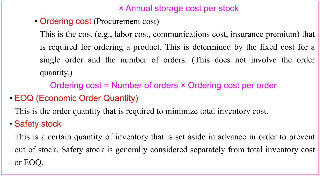
Source visual description
Original source visual. Selectable source labels and wording: × Annual storage cost per stock • Ordering cost (Procurement cost) This is the cost (e.g., labor cost, communications cost, insurance premium) that is required for ordering a product. This is determined by the fixed cost for a single order and the number of orders. (This does not involve the order quantity.) Ordering cost = Number of orders × Ordering cost per order • EOQ (Economic Order Quantity) This is the order quantity that is required to minimize total inventory cost. • Safety stock This is a certain quantity of inventory that is set aside in advance in order to prevent out of stock. Safety stock is generally considered separately from total inventory cost or EOQ.
Original visual text
× Annual storage cost per stock • Ordering cost (Procurement cost) This is the cost (e.g., labor cost, communications cost, insurance premium) that is required for ordering a product. This is determined by the fixed cost for a single order and the number of orders. (This does not involve the order quantity.) Ordering cost = Number of orders × Ordering cost per order • EOQ (Economic Order Quantity) This is the order quantity that is required to minimize total inventory cost. • Safety stock This is a certain quantity of inventory that is set aside in advance in order to prevent out of stock. Safety stock is generally considered separately from total inventory cost or EOQ.
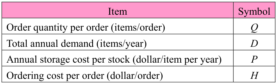
If the single order quantity is increased, the average inventory quantity will increase along with the storage cost. If it is decreased, the number of orders will increase along with the ordering cost. With this in mind, the following explains how to calculate EOQ (Economic Order Quantity). Each item in this explanation is written by using the following symbols.
| Item | Symbol |
|---|---|
| Order quantity per order (items/order) | Q |
| Total annual demand (items/year) | D |
| Annual storage cost per stock (dollar/item per year) | P |
| Ordering cost per order (dollar/order) | H |
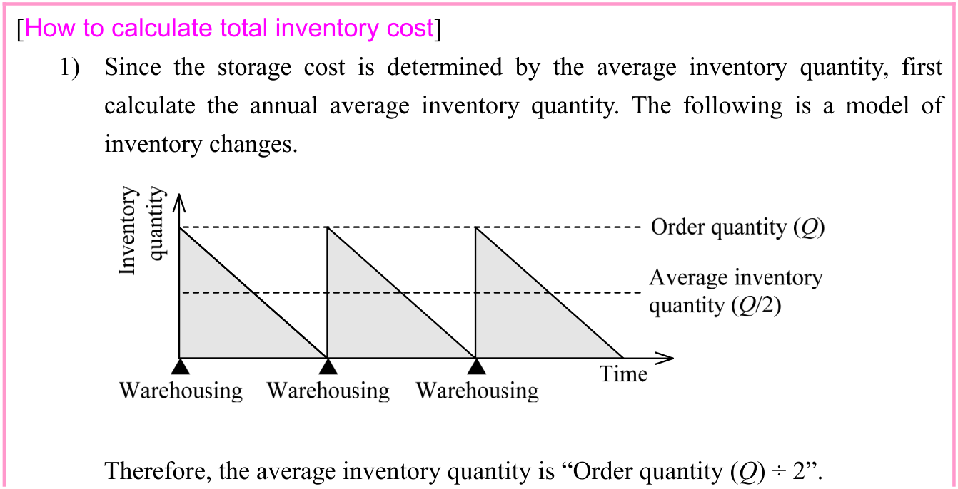
Source visual description
Original source visual. Selectable source labels and wording: [How to calculate total inventory cost] 1) Since the storage cost is determined by the average inventory quantity, first calculate the annual average inventory quantity. The following is a model of inventory changes. Therefore, the average inventory quantity is “Order quantity (Q) ÷ 2”.
Original visual text
[How to calculate total inventory cost] 1) Since the storage cost is determined by the average inventory quantity, first calculate the annual average inventory quantity. The following is a model of inventory changes. Therefore, the average inventory quantity is “Order quantity (Q) ÷ 2”.
p. 64 · PDF 68
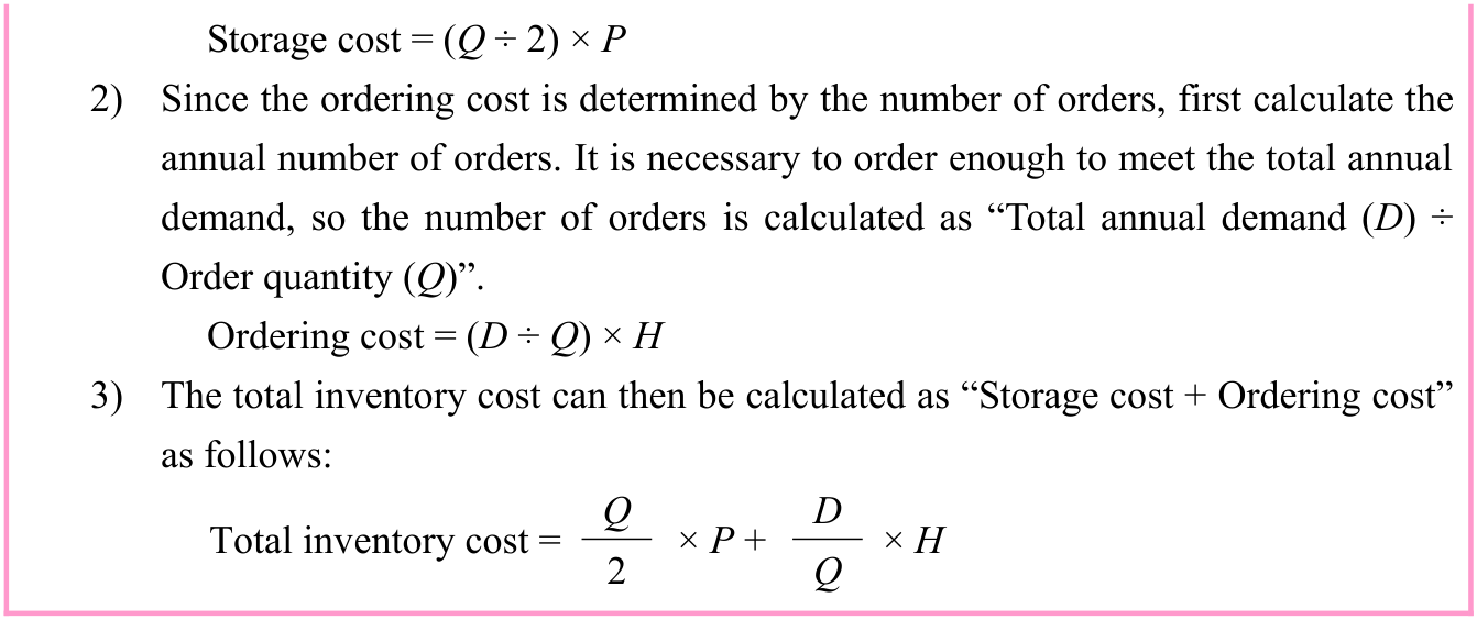
Source visual description
Original source visual. Selectable source labels and wording: Storage cost = (Q ÷ 2) × P 2) Since the ordering cost is determined by the number of orders, first calculate the annual number of orders. It is necessary to order enough to meet the total annual demand, so the number of orders is calculated as “Total annual demand (D) ÷ Order quantity (Q)”. Ordering cost = (D ÷ Q) × H 3) The total inventory cost can then be calculated as “Storage cost + Ordering cost” as follows: Q D Total inventory cost = × P + × H 2 Q
Original visual text
Storage cost = (Q ÷ 2) × P 2) Since the ordering cost is determined by the number of orders, first calculate the annual number of orders. It is necessary to order enough to meet the total annual demand, so the number of orders is calculated as “Total annual demand (D) ÷ Order quantity (Q)”. Ordering cost = (D ÷ Q) × H 3) The total inventory cost can then be calculated as “Storage cost + Ordering cost” as follows: Q D Total inventory cost = × P + × H 2 Q
EOQ (Economic Order Quantity) is calculated as the value of Q that minimizes the total inventory cost. Therefore, it is required to differentiate the equation of the total inventory cost and calculate the value of Q where the slope of the tangent is 0 (i.e., the point where the tangent is parallel with the x axis = the bottom of the curve that represents the expression of the total inventory cost.) If the differentiation is too difficult to solve, it may be easier to understand by looking at the relationship between the order quantity and the cost (i.e., storage, cost ordering cost, total inventory cost) on a graph.
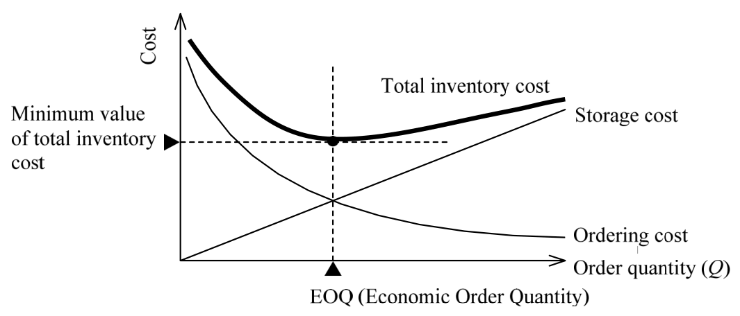
Source visual description
Original inventory-cost graph. The horizontal axis is Order quantity (Q), with Economic order quantity (Q) marked. Curves are Total inventory cost, Storage cost and Ordering cost; a dashed vertical line and horizontal guide identify the Minimum value of total inventory cost.
Original visual text
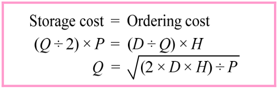
From the graph, it is clear that the point where the total inventory cost is minimized is where the order quantity is “Storage cost = Ordering cost”. Therefore, the EOQ (Economic Order Quantity) value for Q can be calculated as follows:
Source visual description
Original economic-order-quantity derivation box, retaining Storage cost = Ordering cost, the source equality using Q, D, P and H, and the final square-root expression with its original numerator and denominator.
Original visual text
p. 65 · PDF 69
(2) Ordering method
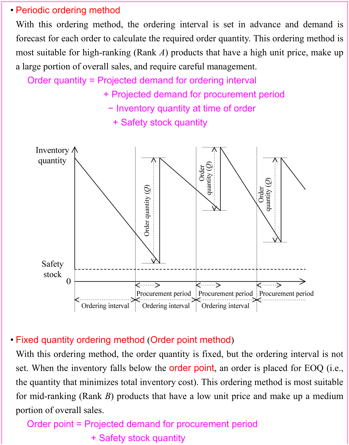
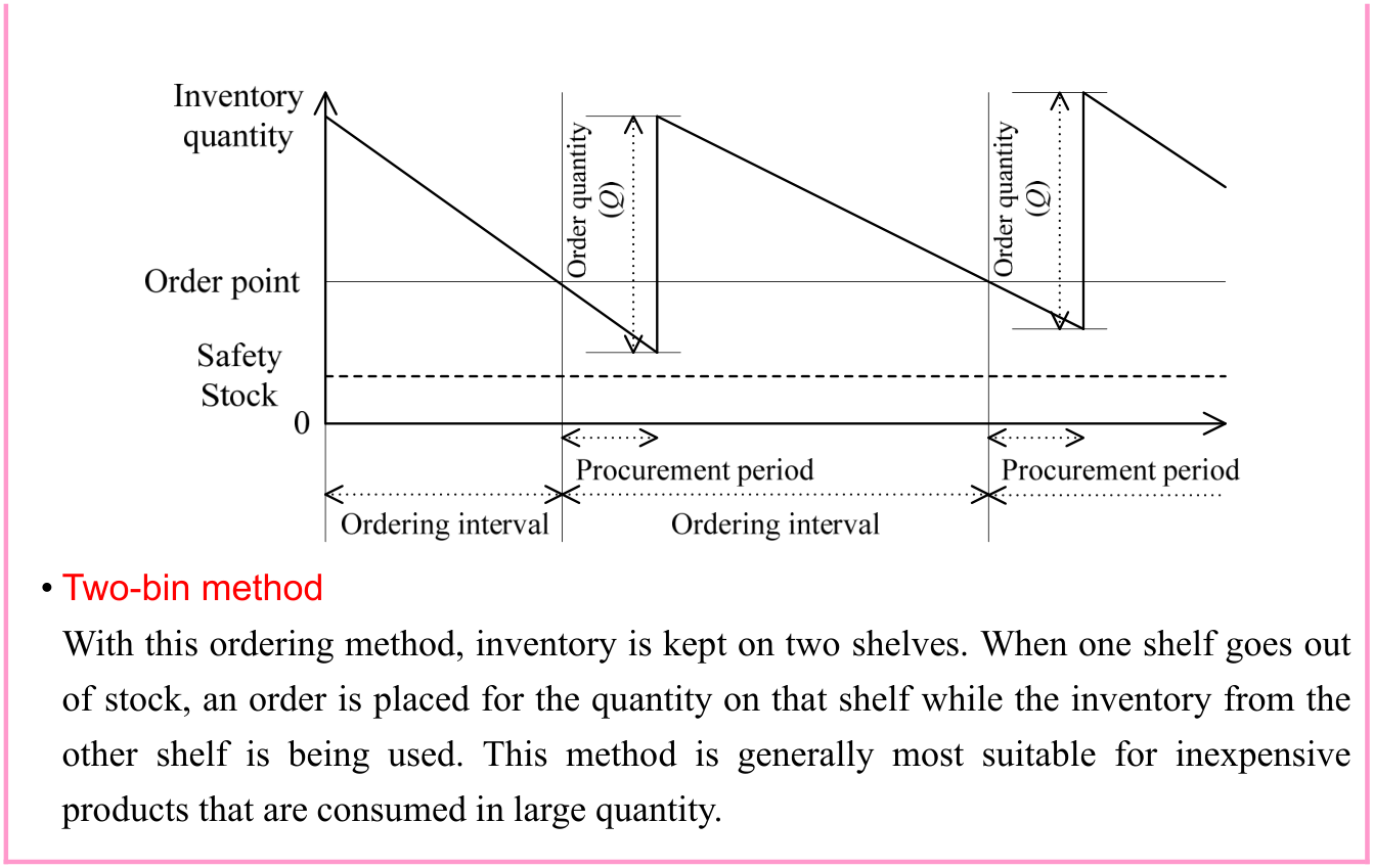
An ordering method is a method that is used to order a product. The ordering method is a vital element in inventory problems. When a product is ordered, it must also consider the procurement period until the ordered product is delivered. Some common ordering methods are listed below.
Source visual description
Original source visual. Selectable source labels and wording: • Periodic ordering method With this ordering method, the ordering interval is set in advance and demand is forecast for each order to calculate the required order quantity. This ordering method is most suitable for high-ranking (Rank A) products that have a high unit price, make up a large portion of overall sales, and require careful management. Order quantity = Projected demand for ordering interval + Projected demand for procurement period − Inventory quantity at time of order + Safety stock quantity • Fixed quantity ordering method (Order point method) With this ordering method, the order quantity is fixed, but the ordering interval is not set. When the inventory falls below the order point, an order is placed for EOQ (i.e., the quantity that minimizes total inventory cost). This ordering method is most suitable for mid-ranking (Rank B) products that have a low unit price and make up a medium portion of overall sales. Order point = Projected demand for procurement period + Safety stock quantity
Original visual text
• Periodic ordering method With this ordering method, the ordering interval is set in advance and demand is forecast for each order to calculate the required order quantity. This ordering method is most suitable for high-ranking (Rank A) products that have a high unit price, make up a large portion of overall sales, and require careful management. Order quantity = Projected demand for ordering interval + Projected demand for procurement period − Inventory quantity at time of order + Safety stock quantity • Fixed quantity ordering method (Order point method) With this ordering method, the order quantity is fixed, but the ordering interval is not set. When the inventory falls below the order point, an order is placed for EOQ (i.e., the quantity that minimizes total inventory cost). This ordering method is most suitable for mid-ranking (Rank B) products that have a low unit price and make up a medium portion of overall sales. Order point = Projected demand for procurement period + Safety stock quantity
p. 66 · PDF 70
Source visual description
Original source visual. Selectable source labels and wording: • Two-bin method With this ordering method, inventory is kept on two shelves. When one shelf goes out of stock, an order is placed for the quantity on that shelf while the inventory from the other shelf is being used. This method is generally most suitable for inexpensive products that are consumed in large quantity.
Original visual text
• Two-bin method With this ordering method, inventory is kept on two shelves. When one shelf goes out of stock, an order is placed for the quantity on that shelf while the inventory from the other shelf is being used. This method is generally most suitable for inexpensive products that are consumed in large quantity.
3-2-4 Demand Forecasting
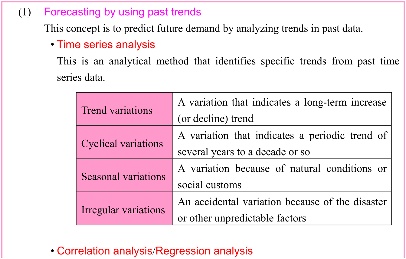
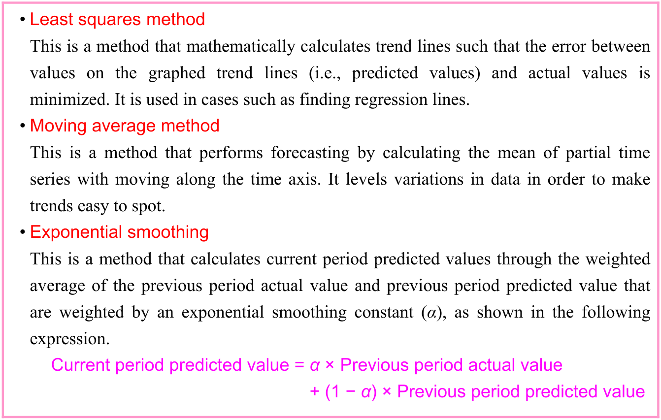
Demand forecasting is the advance forecasting of future demand in order to make product manufacturing plans and order plans. The following are three approaches for a concept of demand forecasting.
Source visual description
Original source visual. Selectable source labels and wording: Forecasting by using past trends (1) This concept is to predict future demand by analyzing trends in past data. • Time series analysis This is an analytical method that identifies specific trends from past time series data. A variation that indicates a long-term increase Trend variations (or decline) trend A variation that indicates a periodic trend of Cyclical variations several years to a decade or so A variation because of natural conditions or Seasonal variations social customs An accidental variation because of the disaster Irregular variations or other unpredictable factors • Correlation analysis/Regression analysis
Original visual text
Forecasting by using past trends (1) This concept is to predict future demand by analyzing trends in past data. • Time series analysis This is an analytical method that identifies specific trends from past time series data. A variation that indicates a long-term increase Trend variations (or decline) trend A variation that indicates a periodic trend of Cyclical variations several years to a decade or so A variation because of natural conditions or Seasonal variations social customs An accidental variation because of the disaster Irregular variations or other unpredictable factors • Correlation analysis/Regression analysis
p. 67 · PDF 71
This is a method that analyzes correlation between cause and effect in past actual demand. A correlation coefficient is calculated by correlation analysis to study the strength of associations, while a regression line is calculated by regression analysis to use for demand forecasting.
(2) Forecasting by using current index This is a concept to forecast future demand from index currently in use. It includes the cross-section method that makes comparisons with data for similar products at the same points in time in the past, and the leading indicator method that identifies index to indicate future trends on the basis of statistical data.
(3) Forecasting by using models This is a concept to create and analyze models for forecasting future demand. It includes econometric analysis that finds solutions to modeled prediction equations (i.e., simultaneous equations), and inter-industry analysis that creates linear programming models by using inter-industry relations tables.
The following are also methods for demand forecasting.
Source visual description
Original source visual. Selectable source labels and wording: • Least squares method This is a method that mathematically calculates trend lines such that the error between values on the graphed trend lines (i.e., predicted values) and actual values is minimized. It is used in cases such as finding regression lines. • Moving average method This is a method that performs forecasting by calculating the mean of partial time series with moving along the time axis. It levels variations in data in order to make trends easy to spot. • Exponential smoothing This is a method that calculates current period predicted values through the weighted average of the previous period actual value and previous period predicted value that are weighted by an exponential smoothing constant (α), as shown in the following expression. Current period predicted value = α × Previous period actual value + (1 − α) × Previous period predicted value
Original visual text
• Least squares method This is a method that mathematically calculates trend lines such that the error between values on the graphed trend lines (i.e., predicted values) and actual values is minimized. It is used in cases such as finding regression lines. • Moving average method This is a method that performs forecasting by calculating the mean of partial time series with moving along the time axis. It levels variations in data in order to make trends easy to spot. • Exponential smoothing This is a method that calculates current period predicted values through the weighted average of the previous period actual value and previous period predicted value that are weighted by an exponential smoothing constant (α), as shown in the following expression. Current period predicted value = α × Previous period actual value + (1 − α) × Previous period predicted value
3-2-5 Game Theory
Game theory is a technique to consider the optimal strategy for a player to win a game. In corporate activities, it is used to identify the most effective future strategy from among
p. 68 · PDF 72
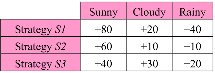
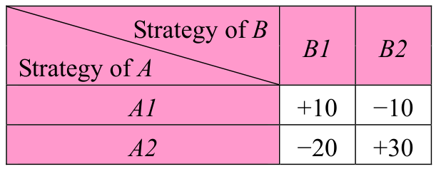
multiple possible strategies. In game theory, strategy is determined by representing the profit or loss of strategies with the following payoff table (payoff matrix).
[Payoff table (1)]
[Payoff table (2)]
| Sunny | Cloudy | Rainy | |
|---|---|---|---|
| Strategy S1 | +80 | +20 | −40 |
| Strategy S2 | +60 | +10 | −10 |
| Strategy S3 | +40 | +30 | −20 |
Source visual description
Original Original source table, printed page 68, region 1. Original selectable labels and wording: Strategy of B Strategy of A B1 B2 A1 +10 −10 A2 −20 +30
Original visual text
Strategy of B B1 B2 Strategy of A A1 +10 −10 A2 −20 +30
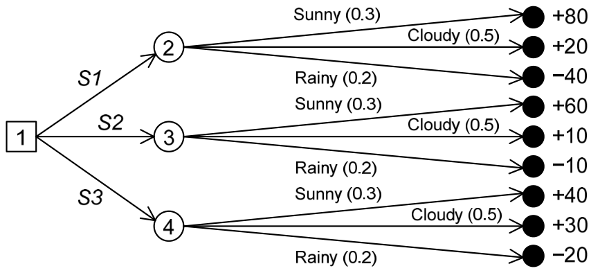
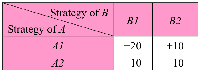
Payoff table (1) shows the benefit that varies with the tomorrow’s weather when a company has selected one of strategies S1 though S3. On the other hand, payoff table (2) shows how the benefit to company A varies with the strategy (B1 or B2) that is selected by company B, when company A has selected strategy A1 or A2. In this case, a profit for company A is a loss for company B, and a loss for company A is a profit for company B. (Such a game is called a two-player zero-sum game.)
When a strategy is determined, it is not possible to perfectly predict future conditions. In response, strategy is determined on the basis of criteria for judging future uncertainty. Criteria for judging future uncertainty can be divided into the following three cases.
- • Definite future
Future conditions are known in advance, or specific conditions can be seen as coming about. - • Probable future
A certain number of future conditions can be imagined, with a known probability of each condition occurring. - • Indefinite future
A certain number of future conditions can be imagined, although which conditions will come about is a complete unknown.
When the future is a definite one, the optimal strategy can be taken for the conditions that can be expected. For example, if it is known that tomorrow’s weather will be sunny in payoff table (1), then the maximum profit of +80 can be obtained by selecting strategy S1. Moreover, if it is known that company B will surely select strategy B1 in payoff table (2), a maximum profit of +10 can be obtained by selecting strategy A1. However, cases in which the future is a definite one are rare. Since the future is often a probable or indefinite one, some judgment criteria are used to determine strategies.
p. 69 · PDF 73
(1) In the case of probable future
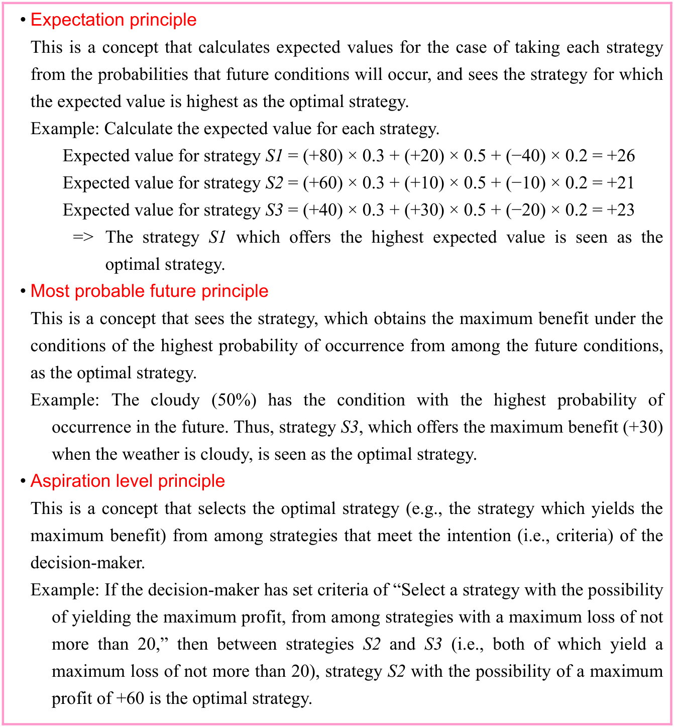
The judgment criteria for the case of a probable future are explained in payoff table (1) as a 30% probability that tomorrow’s weather will be sunny, a 50% probability that it will be cloudy, and a 20% probability that it will rain.
Source visual description
Original source visual. Selectable source labels and wording: • Expectation principle This is a concept that calculates expected values for the case of taking each strategy from the probabilities that future conditions will occur, and sees the strategy for which the expected value is highest as the optimal strategy. Example: Calculate the expected value for each strategy. Expected value for strategy S1 = (+80) × 0.3 + (+20) × 0.5 + (−40) × 0.2 = +26 Expected value for strategy S2 = (+60) × 0.3 + (+10) × 0.5 + (−10) × 0.2 = +21 Expected value for strategy S3 = (+40) × 0.3 + (+30) × 0.5 + (−20) × 0.2 = +23 => The strategy S1 which offers the highest expected value is seen as the optimal strategy. • Most probable future principle This is a concept that sees the strategy, which obtains the maximum benefit under the conditions of the highest probability of occurrence from among the future conditions, as the optimal strategy. Example: The cloudy (50%) has the condition with the highest probability of occurrence in the future. Thus, strategy S3, which offers the maximum benefit (+30) when the weather is cloudy, is seen as the optimal strategy. • Aspiration level principle This is a concept that selects the optimal strategy (e.g., the strategy which yields the maximum benefit) from among strategies that meet the intention (i.e., criteria) of the decision-maker. Example: If the decision-maker has set criteria of “Select a strategy with the possibility of yielding the maximum profit, from among strategies with a maximum loss of not more than 20,” then between strategies S2 and S3 (i.e., both of which yield a maximum loss of not more than 20), strategy S2 with the possibility of a maximum profit of +60 is the optimal strategy.
Original visual text
• Expectation principle This is a concept that calculates expected values for the case of taking each strategy from the probabilities that future conditions will occur, and sees the strategy for which the expected value is highest as the optimal strategy. Example: Calculate the expected value for each strategy. Expected value for strategy S1 = (+80) × 0.3 + (+20) × 0.5 + (−40) × 0.2 = +26 Expected value for strategy S2 = (+60) × 0.3 + (+10) × 0.5 + (−10) × 0.2 = +21 Expected value for strategy S3 = (+40) × 0.3 + (+30) × 0.5 + (−20) × 0.2 = +23 => The strategy S1 which offers the highest expected value is seen as the optimal strategy. • Most probable future principle This is a concept that sees the strategy, which obtains the maximum benefit under the conditions of the highest probability of occurrence from among the future conditions, as the optimal strategy. Example: The cloudy (50%) has the condition with the highest probability of occurrence in the future. Thus, strategy S3, which offers the maximum benefit (+30) when the weather is cloudy, is seen as the optimal strategy. • Aspiration level principle This is a concept that selects the optimal strategy (e.g., the strategy which yields the maximum benefit) from among strategies that meet the intention (i.e., criteria) of the decision-maker. Example: If the decision-maker has set criteria of “Select a strategy with the possibility of yielding the maximum profit, from among strategies with a maximum loss of not more than 20,” then between strategies S2 and S3 (i.e., both of which yield a maximum loss of not more than 20), strategy S2 with the possibility of a maximum profit of +60 is the optimal strategy.
In the case of a probable future, a decision tree, such as the following, may be used. In a
decision tree, decision-making that is represented with □ (decision node) and indefinite events that are represented with ○ (chance node) are numbered in order. Those nodes are to
be options through linking logically and in time series, and the outcomes of options are
written in end nodes that are represented with ●.
p. 70 · PDF 74
Source visual description
Original decision tree for the probable-future example. Branches retain strategies S1, S2 and S3, weather Sunny, Cloudy and Rainy, original probabilities, outcome amounts and the source decision/chance node symbols.
Original visual text
(2) In the case of indefinite future
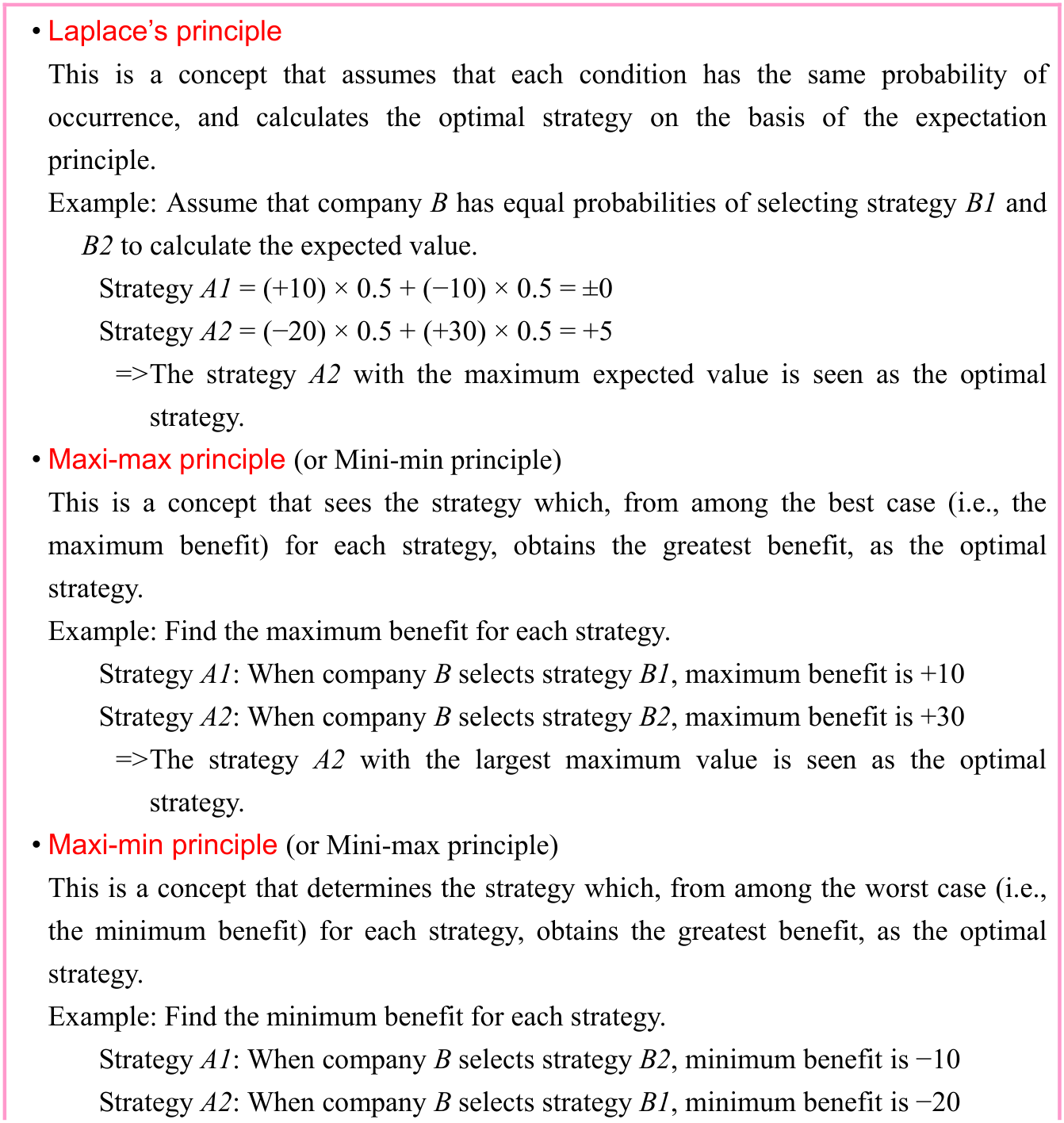
Judgment criteria for the case of indefinite future are explained in payoff table (2).
Source visual description
Original source visual. Selectable source labels and wording: • Laplace’s principle This is a concept that assumes that each condition has the same probability of occurrence, and calculates the optimal strategy on the basis of the expectation principle. Example: Assume that company B has equal probabilities of selecting strategy B1 and B2 to calculate the expected value. Strategy A1 = (+10) × 0.5 + (−10) × 0.5 = ±0 Strategy A2 = (−20) × 0.5 + (+30) × 0.5 = +5 => The strategy A2 with the maximum expected value is seen as the optimal strategy. • Maxi-max principle (or Mini-min principle) This is a concept that sees the strategy which, from among the best case (i.e., the maximum benefit) for each strategy, obtains the greatest benefit, as the optimal strategy. Example: Find the maximum benefit for each strategy. Strategy A1: When company B selects strategy B1, maximum benefit is +10 Strategy A2: When company B selects strategy B2, maximum benefit is +30 => The strategy A2 with the largest maximum value is seen as the optimal strategy. • Maxi-min principle (or Mini-max principle) This is a concept that determines the strategy which, from among the worst case (i.e., the minimum benefit) for each strategy, obtains the greatest benefit, as the optimal strategy. Example: Find the minimum benefit for each strategy. Strategy A1: When company B selects strategy B2, minimum benefit is −10 Strategy A2: When company B selects strategy B1, minimum benefit is −20
Original visual text
• Laplace’s principle This is a concept that assumes that each condition has the same probability of occurrence, and calculates the optimal strategy on the basis of the expectation principle. Example: Assume that company B has equal probabilities of selecting strategy B1 and B2 to calculate the expected value. Strategy A1 = (+10) × 0.5 + (−10) × 0.5 = ±0 Strategy A2 = (−20) × 0.5 + (+30) × 0.5 = +5 => The strategy A2 with the maximum expected value is seen as the optimal strategy. • Maxi-max principle (or Mini-min principle) This is a concept that sees the strategy which, from among the best case (i.e., the maximum benefit) for each strategy, obtains the greatest benefit, as the optimal strategy. Example: Find the maximum benefit for each strategy. Strategy A1: When company B selects strategy B1, maximum benefit is +10 Strategy A2: When company B selects strategy B2, maximum benefit is +30 => The strategy A2 with the largest maximum value is seen as the optimal strategy. • Maxi-min principle (or Mini-max principle) This is a concept that determines the strategy which, from among the worst case (i.e., the minimum benefit) for each strategy, obtains the greatest benefit, as the optimal strategy. Example: Find the minimum benefit for each strategy. Strategy A1: When company B selects strategy B2, minimum benefit is −10 Strategy A2: When company B selects strategy B1, minimum benefit is −20
p. 71 · PDF 75
Source visual description
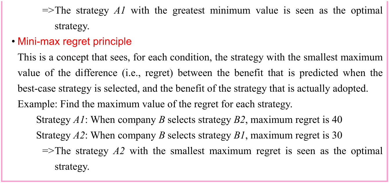
Original source visual. Selectable source labels and wording: => The strategy A1 with the greatest minimum value is seen as the optimal strategy. • Mini-max regret principle This is a concept that sees, for each condition, the strategy with the smallest maximum value of the difference (i.e., regret) between the benefit that is predicted when the best-case strategy is selected, and the benefit of the strategy that is actually adopted. Example: Find the maximum value of the regret for each strategy. Strategy A1: When company B selects strategy B2, maximum regret is 40 Strategy A2: When company B selects strategy B1, maximum regret is 30 => The strategy A2 with the smallest maximum regret is seen as the optimal strategy.
Original visual text
=> The strategy A1 with the greatest minimum value is seen as the optimal strategy. • Mini-max regret principle This is a concept that sees, for each condition, the strategy with the smallest maximum value of the difference (i.e., regret) between the benefit that is predicted when the best-case strategy is selected, and the benefit of the strategy that is actually adopted. Example: Find the maximum value of the regret for each strategy. Strategy A1: When company B selects strategy B2, maximum regret is 40 Strategy A2: When company B selects strategy B1, maximum regret is 30 => The strategy A2 with the smallest maximum regret is seen as the optimal strategy.
Source visual description
Original Original source table, printed page 71, region 2. Original selectable labels and wording: Strategy of B Strategy of A B1 B2 A1 +20 +10 A2 +10 −10
Original visual text
Strategy of B B1 B2 Strategy of A A1 +20 +10 A2 +10 −10
In the case of a payoff table such as that at
right, no matter which strategy company B
selects, company A is better off by selecting
strategy A1. A strategy such as A1 is called a
dominant strategy (or superiority strategy).
3-2-6 Optimization Problems
Optimization problems are those problems which identify solutions that are best cases for specified conditions. Linear programming, scheduling, and inventory planning, which have been explained earlier, are optimization problems. The following are two approaches to optimization problems.
- • Divide-and-conquer approach
This is a method that divides large and complex problems into small problems, and solves each of these to find a solution to the overall problem. It can be seen as a top-down approach that splits up problems from the whole into parts. - • Dynamic programming
This is a method that solves large and complex problems by beginning with parts for which optimal solutions can be fixed, to in the end find a solution to the overall problem. It can be seen as a bottom-up approach that integrates problems from parts into an overall solution.
The following example will consider a shortest path problem to find how many paths of the shortest ones from A to B in the diagram pass through X.
p. 72 · PDF 76
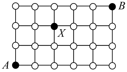
Source visual description
Original shortest-path grid with A at the lower left, B at the upper right and intermediate X. All lattice nodes, paths and the marked A-X-B points are preserved.
Original visual text
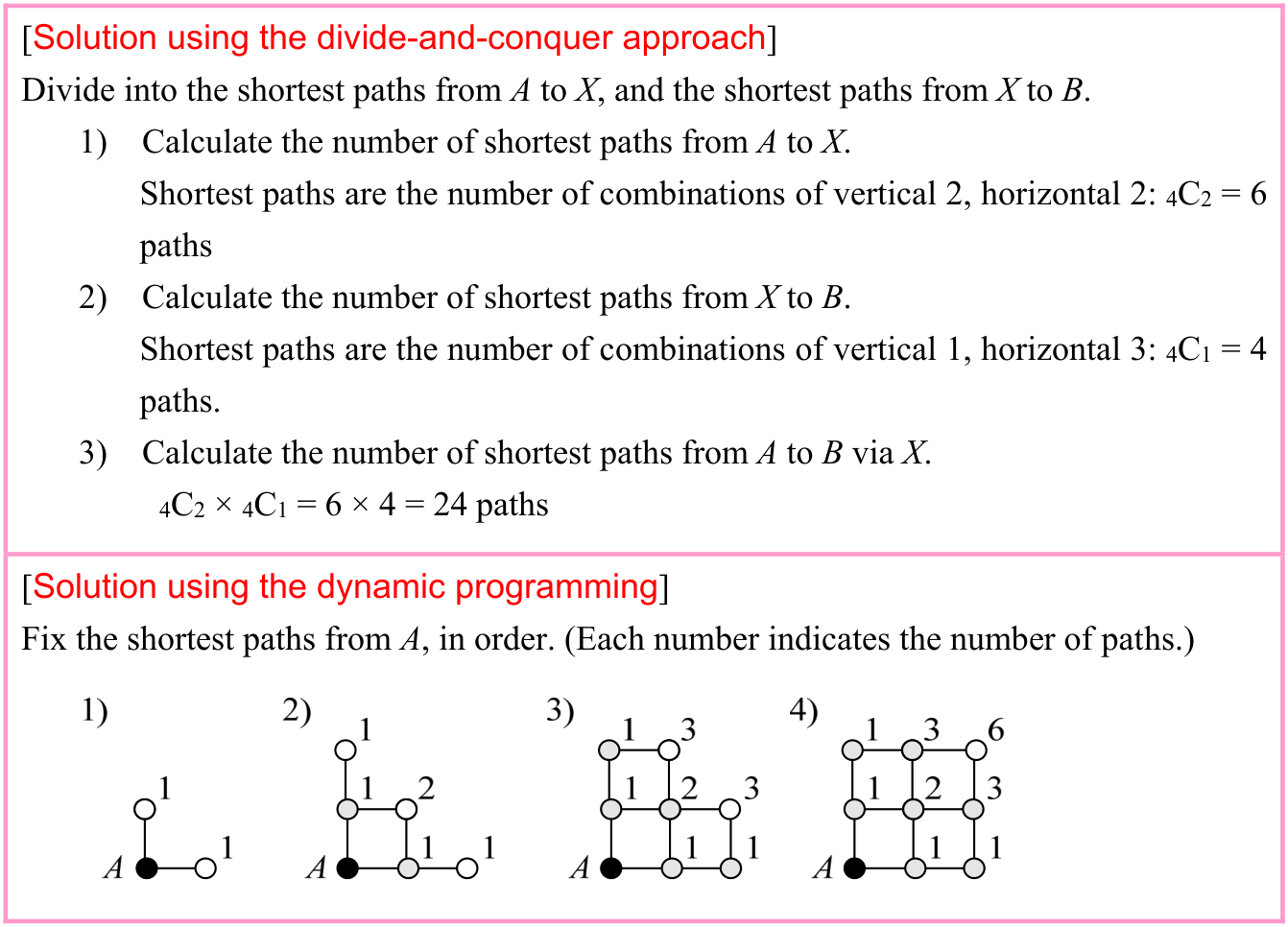
Source visual description
Original paired shortest-path solutions. The divide-and-conquer solution retains the two combination calculations, 6 paths and 4 paths, and their product 24. The dynamic-programming solution retains the numbered incremental grids and every original node count.
Original visual text
[Solution using the divide-and-conquer approach] Divide into the shortest paths from A to X, and the shortest paths from X to B. 1) Calculate the number of shortest paths from A to X. Shortest paths are the number of combinations of vertical 2, horizontal 2: 4C2 = 6 paths 2) Calculate the number of shortest paths from X to B. Shortest paths are the number of combinations of vertical 1, horizontal 3: 4C1 = 4 paths. 3) Calculate the number of shortest paths from A to B via X. 4C2 × 4C1 = 6 × 4 = 24 paths [Solution using the dynamic programming] Fix the shortest paths from A, in order. (Each number indicates the number of paths.)
Section progress
Original chapter exercises
Original chapter exercises →New FE Textbook Vol.2 · First Edition, April 2015