p. 425 · PDF 435

2-2-4 Computational Complexity

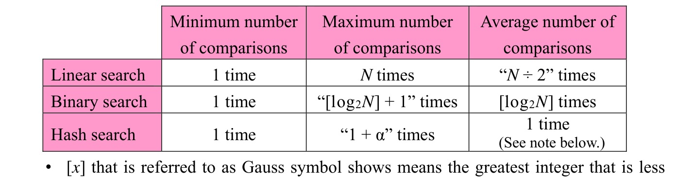
Computational complexity is one of the indicators for evaluating algorithms. There is time complexity which shows the increase in processing time according to the amount of data to be processed, and space complexity which shows the increase in the use of memory space. The notation system of computational complexity includes big O notation which shows the upper limit of computational complexity of an algorithm with O (i.e., order). In the big O notation, if computational complexity of the part that has the maximum impact on the overall is proportional to data number N, it is represented as O(N). If it is proportional to the square of N, it is represented as O(N²). The computational complexity (e.g., time complexity) for three search algorithms is compared. In a search algorithm, a comparison process (decision process) is repeated until the target value is found. Therefore, the number of comparisons (i.e., number of searches) decides the processing time of the algorithm (or the implemented program). The following is the number of comparisons made in each search algorithm for N data items that are covered in the search.

Enlarge original visual

Original source text

Minimum number 
Maximum number 
Average number of 
of comparisons 
of comparisons 
comparisons 
Linear search 
1 time 
N times 
“N ÷ 2” times 
Binary search 
1 time 
“[log2N] + 1” times
[log2N] times 
1 time 
Hash search  
1 time 
“1 + α” times 
(See note below.) 
• [x] that is referred to as Gauss symbol shows means the greatest integer that is less 

Source visual description

Original Computational Complexity source layout. Source labels: Minimum number; of comparisons; Maximum number; of comparisons; Average number of.

p. 426 · PDF 436

than or equal to x.

• • log2N shows x for which 2^x = N (e.g., log216 = 4).
  Note: This is the case the storage location (i.e., hash value) is approximated with uniform distribution, and in addition, the probability of occurrence of a synonym is so small that it can be ignored.

Enlarge original visual

Original source text

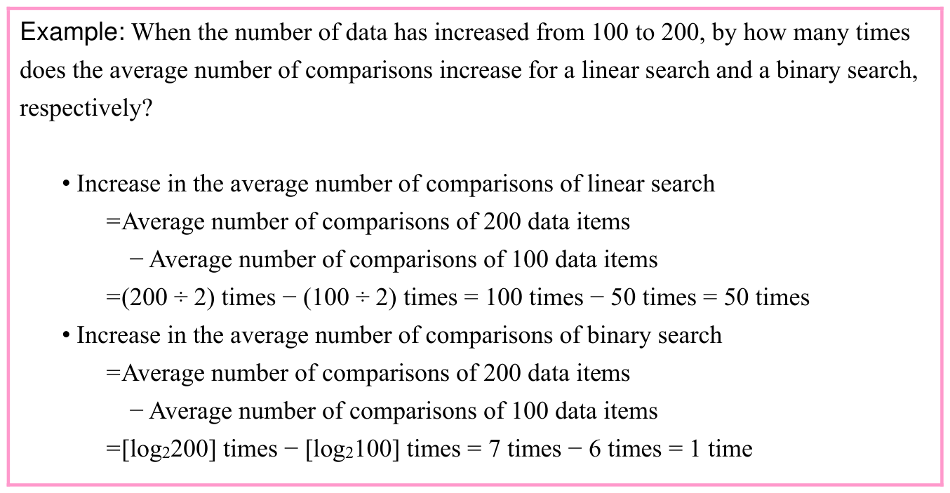
Example: When the number of data has increased from 100 to 200, by how many times 
does the average number of comparisons increase for a linear search and a binary search, 
respectively? 
• Increase in the average number of comparisons of linear search 
= Average number of comparisons of 200 data items  
− Average number of comparisons of 100 data items 
= (200 ÷ 2) times − (100 ÷ 2) times = 100 times − 50 times = 50 times 
• Increase in the average number of comparisons of binary search 
= Average number of comparisons of 200 data items  
− Average number of comparisons of 100 data items 
= [log2200] times − [log2100] times = 7 times − 6 times = 1 time 

Source visual description

Original Computational Complexity source layout. Source labels: Example: When the number of data has increased from 100 to 200, by how many times; does the average number of comparisons increase for a linear search and a binary search,; respectively?; • Increase in the average number of comparisons of linear search; = Average number of comparisons of 200 data items.

Therefore, the computational complexity of linear search is O(N), computational the complexity of binary search is O(log2N), and the computation complexity of hash search is O(1). The computational complexity of big O notation is an indicator (or rough guide), and it may not always match with the actual processing time. For example, when the target value is not found, the maximum number of comparisons is made. Therefore, the average search time varies depending on the probability of search success and search failure. If an improvement is made so that the search ends as soon as it is known that the target value does not exist by using the data recorded in ascending order (or descending order) in linear search, the number of comparisons can be reduced in the event of search failure. However, the order does not change. · 1 question